20251014-csprimer-algorithms

csprimer-algorithms

002 Convert to Roman

1. understand the problem
2. start from smaller problem
3. found pattern, solve by recursions or loop etc
4. create your own test, think line by line?

plan:

recursively → substract the larger problem → smaller

scratch and keep planing:

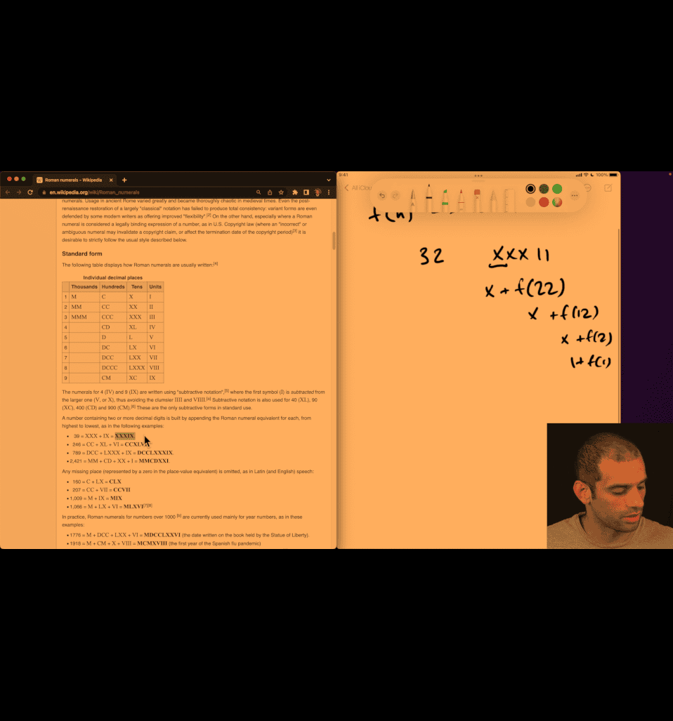
def f(n):
  for d,r:
    if d<=n:
      return r+f(n-d)
  return ""
 

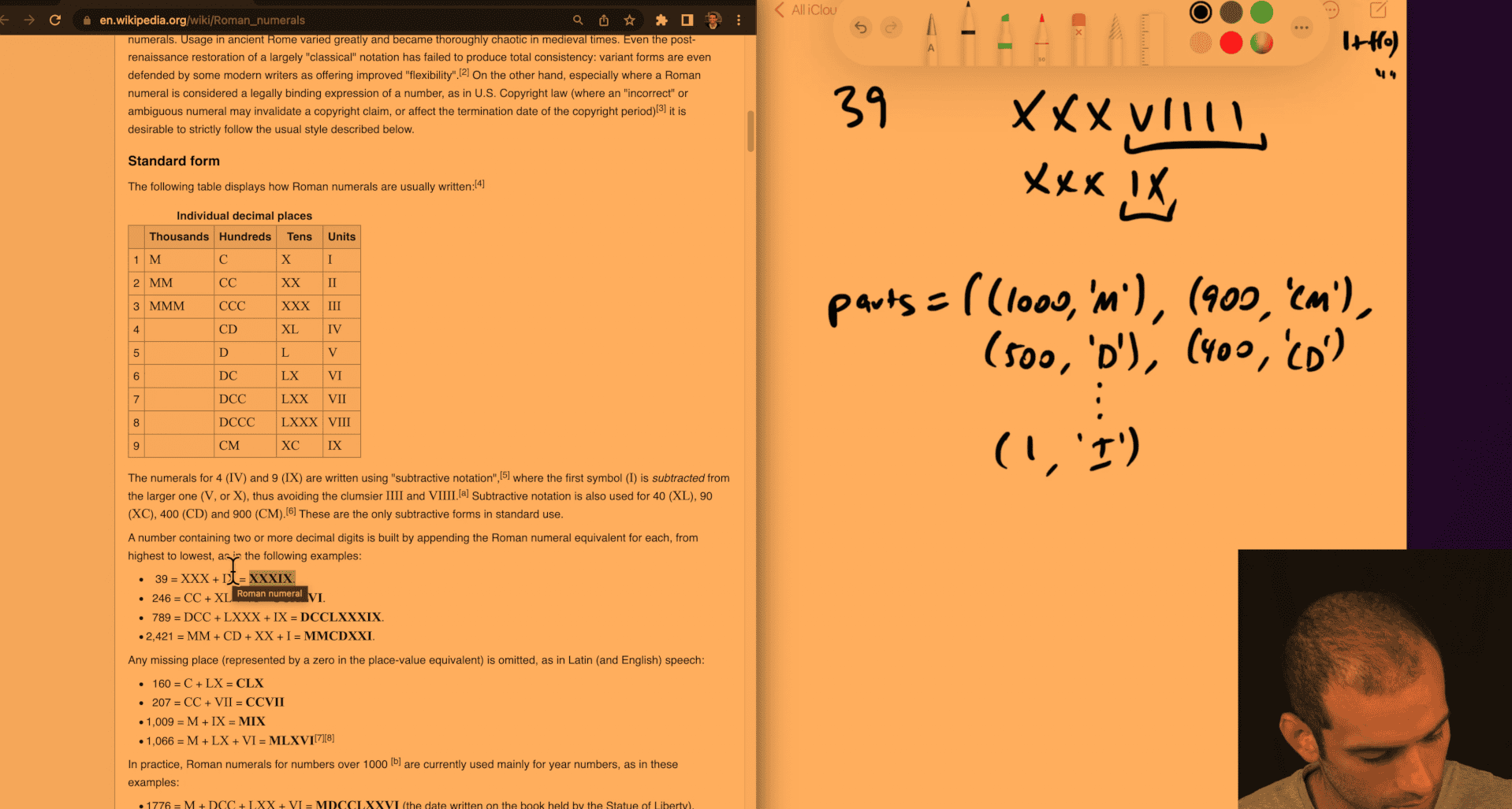
parts = [
    (1000, "M"),
    (900, "CM"),
    (500, "D"),
    (400, "CD"),
    (100, "C"),
    (90, "XC"),
    (50, "L"),
    (40, "XL"),
    (10, "X"),
    (9, "IX"),
    (5, "V"),
    (4, "IV"),
    (1, "I"),
]
 
 
def f(n):
    if n <= 0:
        return ""
    for d, r in parts:
        if d <= n:
            return r + f(n - d)
    return ""
 
if __name__ == "__main__":
    cases = ((39, "XXXIX"), (2421, "MMCDXXI"), (1066, "MLXVI"))
    for n, x in cases:
        assert f(n) == x
    print("ok")

more overkill feature: binary search bisect

from bisect import bisect_right
 
values = [1, 4, 5, 9, 10, 40, 50, 90, 100, 400, 500, 900, 1000]
symbols = ["I", "IV", "V", "IX", "X", "XL", "L", "XC", "C", "CD", "D", "CM", "M"]
 
 
def f(n):
    r = ""
    while n > 0:
        i = bisect_right(values, n) - 1  # largest value <= n
        r += symbols[i]
        n -= values[i]
    return r
 

---

003 Correct binary search.mp4

from typing import List, Optional
 
def binsearch(nums: List[int], target: int) -> Optional[int]:
    lo = 0
    hi = len(nums) - 1
    # Invariant: if target is in nums, then it is within indices [lo, hi]
    while lo <= hi:
        mid = lo + (hi - lo) // 2  # avoids overflow and biases toward lower mid
        value = nums[mid]
        if value == target:
            return mid
        if value < target:
            lo = mid + 1  # target, if present, is in [mid+1, hi]
        else:
            hi = mid - 1  # target, if present, is in [lo, mid-1]
    return None
 
#if name=main:
a = [-5, -2, 0]
b = [0, 2, 3, 4, 9]
 
cases = [
    (a, -5, 0),
    (a, -2, 1),
    (a,  0, 2),
    (a,  2, None),
    (a, -3, None),
 
    (b,  0, 0),
    (b,  3, 2),
    (b,  4, 3),
    (b,  2, 1),
    (b,  9, 4),
]
for nums, n, exp in cases:
    assert binsearch(nums, n) == exp, (nums, n, exp, binsearch(nums, n))
print('ok')
 

---

010 The enormous difference between polynomial and exponential.mp4

O(n^2) vs O(2^n)

---

011 Building an intuition for common running times.mp4

• o(n^2) is ok if n ⇐1000 but not for o(2^n)

---

006 Finding duplicates

Asymptotic Analysis and Finding Duplicates

Introduction: Asymptotic Analysis as a Tool

The Love-Hate Relationship

• Many engineers have mixed feelings about Big O notation
• Common issues: under-using and over-using it
• It’s one tool in your toolkit, not the only thing

What Asymptotic Analysis Does

Theoretical perspective:

• Allows speaking about trade-offs between approaches
• Agnostic of the specific system running the code
• Enables algorithms from the 1950s to remain relevant today
• Part of a multi-decade (approaching multi-century) conversation about algorithms

Practical reality:

• You cannot be agnostic of your actual system
• Real systems matter: machine, language, data characteristics, RAM constraints
• Some of the most important decisions depend on context

The balance:

• Theory helps us speak generally and universally
• Practice requires considering the actual system
• Both perspectives are necessary

The Problem: Finding Duplicates

Task: Write a function hasDuplicate(array) that returns true if there are duplicate integers in an array, false otherwise.

Three different engineers propose three different approaches.

Solution 1: Nested Loops (Compare Everything)

Approach

• For each element in the array, compare it to every other element
• Can optimize by using symmetry (comparing A to B but not B to A)

Complexity Analysis

Time: O(n²)

• Work grows as the area of a square (n × n)
• Even with symmetry optimization (comparing only half), it’s still fundamentally n²
• Constant factors (like 1/2) don’t change the complexity class

Space: O(1)

• No extra data structures needed

Growth Example

• Going from 10 to 20 elements: 100 → 400 comparisons
• Going from 10 to 100 elements: 100 → 10,000 comparisons
• Substantial growth as n increases

When to Use

• Simple and straightforward
• Good for small, bounded n
• Easy to understand and maintain
• Not ideal for large databases or unbounded growth

Solution 2: Sort Then Check Adjacent Pairs

Approach

1. Sort the array (non-destructive or sort a copy)
2. Iterate through checking adjacent pairs
3. If any adjacent pair is equal, there’s a duplicate

Complexity Analysis

Time: O(n log n)

• Sorting: O(n log n) - this is “astonishing” because most intuitive sorts are O(n²)
• Iteration: O(n)
• Combined: O(n log n) (the n log n term dominates)

Space: O(n) or O(1)

• O(n) if you need to create a copy (non-destructive)
• O(1) if you can sort in-place

Understanding n log n

Key insight: n log n is much closer to linear than to n²

Concrete examples:

• log₂(1024) = 10 (since 2¹⁰ = 1024)
• log₂(1 billion) ≈ 30 (since 2³⁰ ≈ 1 billion)
• The logarithm grows very slowly compared to n

Comparison:

• For 10,000 elements: iteration takes 10,000 units of work
• n log n is substantially better than n² for large n

When to Use

• Better than O(n²) for large n
• May require extra space if sorting in-place isn’t possible
• More complex than nested loops

Solution 3: Hash Map/Set (Single Pass)

Approach

• Iterate through array once
• For each element, check if it’s already in a hash map/set
• If yes → duplicate found
• If no → add it to the hash map/set

Complexity Analysis

Time: O(n)

• Single pass through array: O(n)
• Hash map operations (insert, lookup): O(1) average case
• Combined: O(n)

Space: O(n)

• Must store all elements in the hash map
• Space grows proportionally with input size

Comparison to Solution 2

Theoretically: O(n) is better than O(n log n)

• There exists some n where Solution 3 is definitely faster

Practically:

• Requires O(n) space (Solution 2 might use O(1) if in-place)
• May not be feasible if RAM is constrained
• More complex than Solution 1

When to Use

• Best theoretical time complexity
• Requires extra space
• Consider: Do we have enough RAM? Is n large enough that the difference matters?

Key Insights About Asymptotic Analysis

What It Discards

1. Constant factors

   • O(n²) vs O(½n²) are the same complexity class
   • The 1/2 optimization doesn’t change the analysis

2. Non-dominant terms

   • O(n log n + n) = O(n log n)
   • The +n term is dominated by n log n

3. Exact counts

   • Focus is on pattern of growth, not precise numbers

Complexity Classes That Matter

In practice, only a handful of complexity classes make a meaningful difference:

• Constant: O(1)
• Linear: O(n)
• Logarithmic: O(log n)
• Linearithmic: O(n log n)
• Polynomial: O(n²), O(n³), etc.
• Exponential: O(2ⁿ) - typically intractable

When Theory Meets Practice

Questions to ask:

1. At what n does this algorithm become too slow?
2. Will our business/database ever reach that n?
3. Is the simpler O(n²) code better if it’s more maintainable?
4. Can we afford the space for the O(n) solution?
5. Is the code maintainable and robust?

Example consideration:

• If checking millions of integers and never trillions
• If O(n²) is fast enough (< 10ms) for your use case
• If simpler code reduces bugs and maintenance cost
• Then: O(n²) might be the right choice

Real-World Application: Database Joins

The three approaches to finding duplicates mirror the three main database join algorithms:

1. Nested Loop Join: O(n²) - compare everything to everything
2. Sort-Merge Join: O(n log n) - sort then merge
3. Hash Join: O(n) - build hash table, probe

This pattern appears in many contexts throughout computer science.

Takeaways

1. Asymptotic analysis is a tool, not the only consideration
2. Theory enables universal conversation about algorithms across decades
3. Practice requires system-specific thinking - machine, data, constraints
4. Simple code can be better if n is bounded and maintainability matters
5. Know when each approach is best:
   • Small n, simple code → O(n²) might be fine
   • Large n, space available → O(n) hash approach
   • Large n, space constrained → O(n log n) sort approach
6. Be able to articulate trade-offs in both theoretical and practical terms
7. This pattern (nested loops, sort, hash) appears everywhere - recognizing it is valuable

Practice Questions

• Beginner: Which approach do you prefer and why?
• Intermediate: When would you prefer each approach over the others?
• Advanced: Find a clear circumstance where each of the three is better than the other two

Notes on Notation

• The speaker uses “O of n” notation but notes that formal Big O definition will be covered separately
• Focus here is on intuitive understanding of growth patterns
• Complexity classes will be covered in more detail in future videos

---

007 Fizzbuzz sum.mp4

Critical question: Do I need to look at every element?

• If yes (e.g., printing FizzBuzz for each number): You’re stuck at O(n)
• If no (e.g., just need the sum): Look for mathematical patterns or closed-form solutions

Within complexity class: You can still optimize constant factors, but for substantial improvement, you need a different complexity class.

with divide and conquer, asking yourself, is there a log time solution to this, would be like saying, could I purchase with divide and conquer, where I divide this into two or more pieces, solve these problems in a way where I can combine the results ?

• the first way that you might want to think about this, you want to try and find a pattern, right, where we can have a mathematical expression for computing that pattern, and so you might

any faster way , pattern?

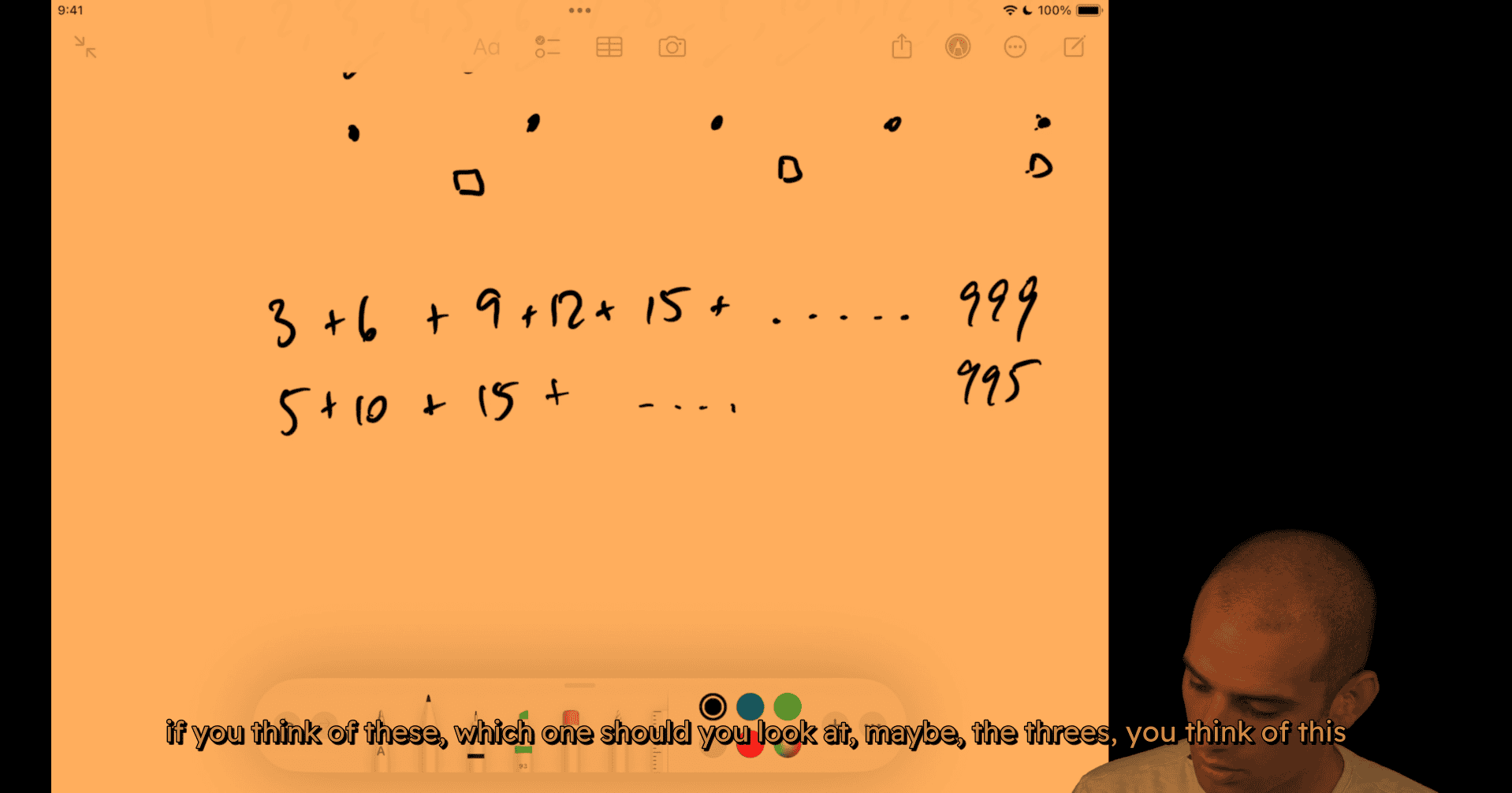
deduct the repeated part (15 common divider for 3 and 5)

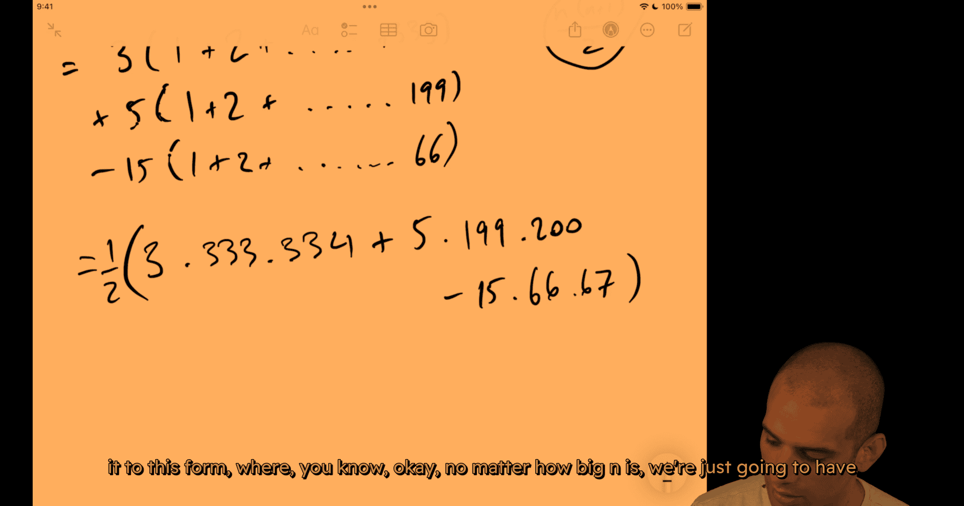
a few multiplications and a few addition subtractions divided by 2, right, n could be billions, constant time solutions

---

008 Just iterate.mp4

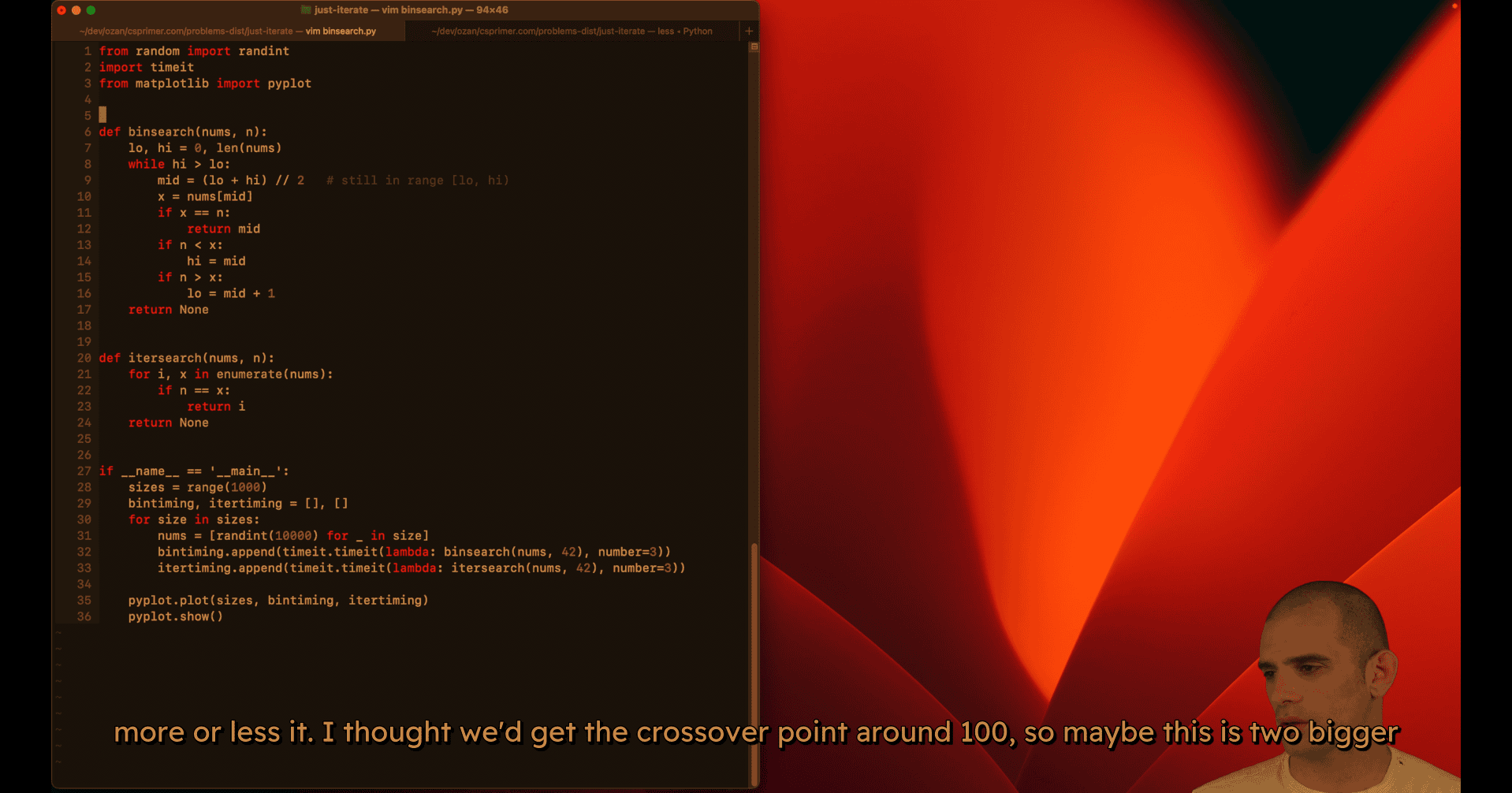
from random import randint
import timeit
from matplotlib import pyplot
 
def binsearch(nums, n):
    lo = 0
    hi = len(nums)
    while hi > lo:
        mid = (lo + hi) // 2  # still in range [lo, hi)
        x = nums[mid]
        if x == n:
            return mid
        if n < x:
            hi = mid
        else:
            lo = mid + 1
    return None
 
def itersearch(nums, n):
    for i, x in enumerate(nums):
        if n == x:
            return i
    return None
 
if __name__ == '__main__':
    sizes = range(200)
    bintiming, itertiming = [], []
    for size in sizes:
        nums = [randint(0, 10000) for _ in range(size)]
        bintiming.append(timeit.timeit(lambda: binsearch(nums, 42), number=3))
        itertiming.append(timeit.timeit(lambda: itersearch(nums, 42), number=3))
    pyplot.plot(sizes, bintiming, itertiming)
    pyplot.show()
 

---

009 Analysis practice.mp4

i just skip the video

• Problem: Cut a 3×3×3 cube into 27 unit cubes with minimum cuts

Asymptotic Analysis: Comprehensive Study Notes

Introduction: The Goal of Asymptotic Analysis

Purpose

• Primary goal: Assess the time and space cost, in Big O terms, of most programs you’ll encounter
• Enable comparison of algorithms in a hardware-agnostic way
• Provide a universal language to discuss algorithms across different systems and contexts
• Balance theoretical understanding with practical systems considerations

The Balance: Theory vs. Practice

Theoretical perspective:

• Allows us to say “this algorithm from the 50s is good” in a universal way
• Makes sense regardless of what machine it’s running on
• Enables conversation about algorithms independent of hardware

Practical reality:

• Cannot ignore hardware, data characteristics, or context
• Cannot ignore maintainability of code
• Need both theoretical and systems understanding

The goal: Be comfortable enough with analysis to proceed to graph search, divide-and-conquer, dynamic programming, and extend analysis techniques to those algorithms.

Core Definition: When Is One Algorithm Better?

The Fundamental Question

Given two algorithms, can we say one is objectively better than the other?

Answer: Yes, if there exists some n where one algorithm definitely outperforms the other, regardless of:

• Constant factors
• Hardware differences (Raspberry Pi vs. supercomputer)
• Boot-up time or initialization overhead

Example

• Algorithm A: Linear time (O(n)) on a slow Raspberry Pi
• Algorithm B: Quadratic time (O(n²)) on a supercomputer

Question: Is A better than B?

Answer: Yes! There exists some n where the linear algorithm on the Raspberry Pi will beat the quadratic algorithm on the supercomputer. Eventually, the growth rate dominates.

Key Insight

• Not for every n, but for some n
• Constant factors don’t matter in the limit
• Hardware differences don’t matter in the limit
• The growth pattern (linear vs. quadratic) is what matters

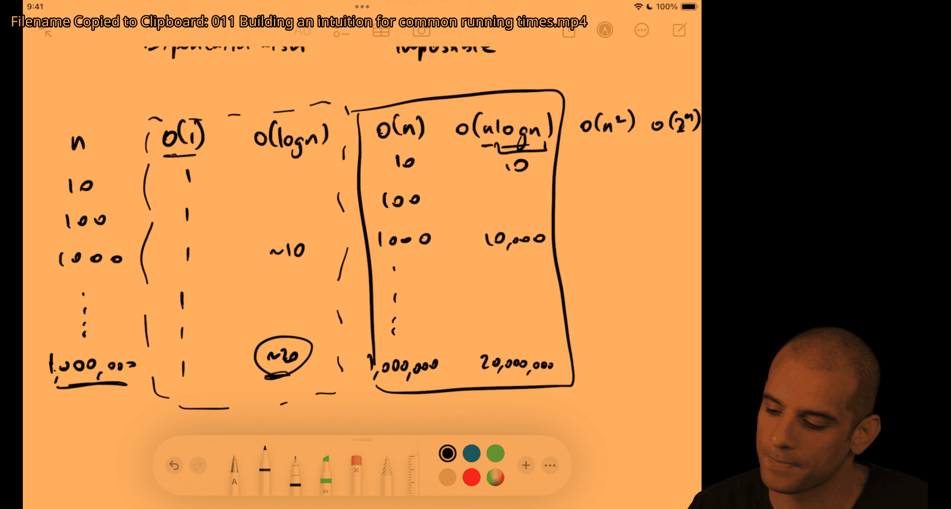
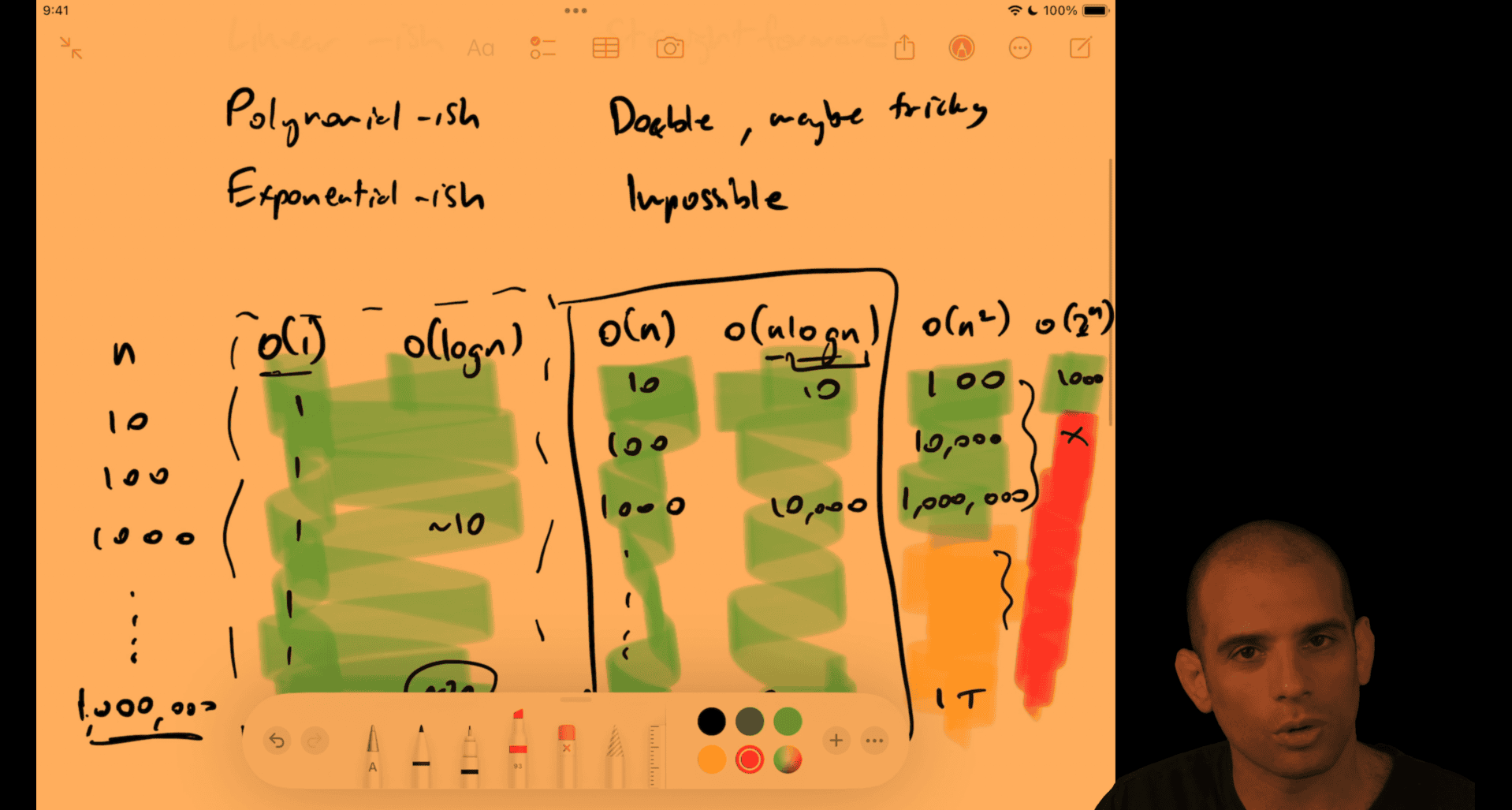
Complexity Classes: The Four Practical Groups

1. Constant-ish

• O(1): Constant time
• O(log n): Logarithmic time
• O(√n): Square root time

Characteristics:

• Effectively “free” or very cheap
• Log n grows extremely slowly (log₂(1000) ≈ 10, log₂(1M) ≈ 20, log₂(1B) ≈ 30)
• Practical systems perspective: these are all “constant-ish”

2. Linear-ish

• O(n): Linear time
• O(n log n): Linearithmic time

Characteristics:

• Scale horizontally: “for every dollar we make, add another server”
• Generally manageable for most applications
• n log n is much closer to linear than to quadratic

3. Polynomial

• O(n²): Quadratic time
• O(n³): Cubic time
• O(nᵏ): Polynomial time for any constant k

Characteristics:

• May need clever optimizations at scale
• At Google scale, might not be affordable
• Generally workable but requires careful consideration

4. Non-Polynomial (Hard Problems)

• O(2ⁿ): Exponential time
• O(n!): Factorial time

Characteristics:

• Effectively impossible for meaningful n
• For exponential: 2⁵⁰ is already intractable
• Cannot use such algorithms in practice

Practical Framing

The four groups help answer:

• Is it effectively free? → Constant-ish
• Can we scale horizontally? → Linear-ish
• Do we need clever optimizations? → Polynomial
• Is it impossible? → Non-polynomial

Units of Measurement

Time Complexity

Unit: Operations

• Could be CPU cycles, seconds, or any consistent unit
• When constant factors are discarded, the exact unit doesn’t matter
• Assumption: Each operation takes consistent time (not always true for big integers, user-defined types, etc.)

Example: Counting function calls

• If each function call takes the same time regardless of input
• Then counting function calls is a valid proxy for time
• Hazard: If function call time varies with input, need to be more careful

Space Complexity

Unit: Memory units

• Could be bytes, stack frames, pages, disk blocks
• Need a consistent unit that grows predictably

Common units:

• Stack frames: For recursive functions, each call uses one stack frame
• Array elements: For data structures, count elements stored
• Bytes: For raw memory usage

Example: Stack space

• Each recursive call pushes a stack frame
• Stack frame size is consistent (contains function locals, return address, etc.)
• Can count stack frames as units of space

Example 1: Constant Time Operations

Simple Multiplication

def multiply(a, b):
    return a * b

Time Complexity: O(1)

• One operation (multiplication)
• Irrespective of input size

Assumptions:

• Integers are primitive types (fit in CPU registers)
• Multiplication is a single CPU instruction
• Not Python big integers (arbitrarily sized)
• Not user-defined types with custom __mul__ methods

When assumptions break:

• Python big integers: multiplication time grows with number size
• Cryptographic operations: multiplying huge primes is not constant
• User-defined types: __mul__ could do anything

Key takeaway: Always consider what assumptions you’re making about input types and operations.

Example 2: Square Root Functions

Built-in Square Root

import math
def sqrt_builtin(n):
    return math.sqrt(n)

Time Complexity: Depends on implementation

• If hardware floating-point: O(1) - constant time
• If software implementation: Could be O(log n) or O(√n)

Binary Search Square Root

def sqrt_binary_search(n):
    # Binary search for k such that k² ≤ n < (k+1)²
    left, right = 1, n
    while left < right:
        mid = (left + right) // 2
        if mid * mid <= n:
            left = mid + 1
        else:
            right = mid
    return left - 1

Time Complexity: O(log n)

• Binary search over space from 1 to n
• Each iteration halves the search space

Linear Search Square Root

def sqrt_linear(n):
    k = 1
    while k * k <= n:
        k += 1
    return k - 1

Time Complexity: O(√n)

• Tries 1², 2², 3², … until finding the answer
• Terminates early at √n iterations

Comparison: O(log n) vs. O(√n)

Theoretical: O(log n) is better (lower complexity class)

Practical considerations:

• Constant factors: Binary search has branch prediction overhead
• Threshold: At n = 64, √64 = 8, log₂(64) = 6
• Real systems: May need to benchmark to determine which is actually faster
• Interview perspective: Want to hear about systems considerations, not just “I’d benchmark”

Key insight: Sometimes O(log n) vs. O(√n) are close enough that constant factors and systems considerations matter more than the theoretical difference.

Example 3: Factorial - Recursive vs. Iterative

Recursive Factorial

def factorial_recursive(n):
    if n <= 1:
        return 1
    return n * factorial_recursive(n - 1)

Time Complexity: O(n)

• Makes n function calls (n, n-1, n-2, …, 1)
• Each call does one multiplication
• Total: n multiplications

Space Complexity: O(n)

• Each recursive call uses one stack frame
• Maximum stack depth: n
• Total: n stack frames

Call chain: Linear chain, not a tree

• factorial(10) → factorial(9) → factorial(8) → … → factorial(1)
• Just a straight line, not branching

Iterative Factorial

def factorial_iterative(n):
    result = 1
    for i in range(1, n + 1):
        result *= i
    return result

Time Complexity: O(n)

• Loop runs n times
• Each iteration: one multiplication
• Total: n multiplications

Space Complexity: O(1)

• Only one accumulator variable
• No stack frames
• Constant space

Comparison

Time: Both O(n) - same asymptotic complexity

Space:

• Recursive: O(n) - stack frames
• Iterative: O(1) - constant space

Practical speed: Iterative is typically faster

• No function call overhead
• No stack frame allocation
• But both are O(n), so this is just a constant factor difference

Tail Call Optimization

What Is Tail Call Optimization?

Tail position: The very last operation in a function, with nothing after it

Tail call: A recursive call in tail position

Tail call optimization (TCO): Compiler/interpreter optimization that converts tail-recursive functions to iterative form automatically

Example: Non-Tail Recursive

def factorial_recursive(n):
    if n <= 1:
        return 1
    return n * factorial_recursive(n - 1)  # NOT tail position

Why not tail?: After the recursive call returns, we still need to multiply by n

Converting to Tail Recursive

def factorial_tail_recursive(n, accumulator=1):
    if n <= 1:
        return accumulator
    return factorial_tail_recursive(n - 1, n * accumulator)  # Tail position

Now it’s tail recursive: The recursive call is the very last thing, nothing happens after it

Benefits of TCO

• Space: O(n) → O(1) (no stack frames needed)
• Speed: Eliminates function call overhead
• Automatic: Compiler/interpreter handles the conversion

Languages with TCO

• LISP: Heavily recursive, TCO is standard
• JavaScript: V8 and other engines support TCO (but not in spec)
• Python: Does NOT support TCO (by design choice)

Key insight: If you can write tail-recursive code, TCO can give you the benefits of iteration (O(1) space) while keeping recursive code structure.

Example 4: Fibonacci - Multiple Approaches

Naive Recursive Fibonacci

def fib_naive(n):
    if n <= 1:
        return n
    return fib_naive(n - 1) + fib_naive(n - 2)

Time Complexity: O(2ⁿ)

• Tree structure: Each call branches into two subproblems
• Height: Approximately n (from n down to base cases)
• Branching factor: 2 (each node has 2 children)
• Total nodes: Approximately 2ⁿ
• Tighter bound exists: But O(2ⁿ) is a valid upper bound

Why exponential?

• fib(10) calls fib(9) and fib(8)
• fib(9) calls fib(8) and fib(7)
• fib(8) is computed twice (once from fib(10), once from fib(9))
• Massive redundant computation

Space Complexity: O(n)

• Stack depth: Maximum depth is n (one path from root to leaf)
• Not O(2ⁿ): Stack shrinks and grows, never exceeds n
• Even though we make 2ⁿ function calls, we don’t need 2ⁿ stack frames simultaneously

Memoized Fibonacci

def fib_memoized(n, memo={}):
    if n in memo:
        return memo[n]
    if n <= 1:
        return n
    memo[n] = fib_memoized(n - 1, memo) + fib_memoized(n - 2, memo)
    return memo[n]

Time Complexity: O(n)

• Unique subproblems: Only n unique values (0, 1, 2, …, n)
• Each computed once: After first computation, cached result is reused
• Total work: n function calls, each doing O(1) work (after memoization)

Space Complexity: O(n)

• Memo cache: Stores n values (0 through n)
• Stack depth: Still O(n) maximum
• Total: O(n) space

Key insight: Memoization eliminates redundant subproblem computation by caching results.

Bottom-Up Dynamic Programming

def fib_bottom_up(n):
    if n <= 1:
        return n
    a, b = 0, 1
    for i in range(2, n + 1):
        a, b = b, a + b
    return b

Time Complexity: O(n)

• Loop runs n-1 times
• Each iteration: constant work (addition, assignment)
• Total: O(n)

Space Complexity: O(1)

• Key insight: Only need the last two values
• State: Two integers (a and b)
• No array needed: Don’t need to store all previous values
• No stack: Iterative, not recursive

Comparison to memoized:

• Time: Both O(n) - same
• Space: Bottom-up is O(1) vs. O(n) for memoized
• Why better?: Recognized that only recent state (last 2 values) is needed

The Progression

1. Naive recursive: O(2ⁿ) time, O(n) space - exponential, unusable
2. Memoized: O(n) time, O(n) space - linear, much better
3. Bottom-up: O(n) time, O(1) space - optimal for this problem

Key lesson: After fixing time complexity, can often optimize space by recognizing what state is actually needed.

Practical Considerations

When Constant Factors Matter

Examples:

• Branch prediction: Binary search has unpredictable branches
• Function call overhead: Recursive calls have overhead
• Cache locality: Array access patterns affect performance
• Memory allocation: Dynamic allocation has overhead

When to benchmark:

• Complexity classes are close (e.g., O(log n) vs. O(√n))
• Constant factors might dominate for your n
• Need to understand systems-level behavior

Not enough to just benchmark: Need to understand why one might be faster/slower to validate your benchmark.

Making Assumptions

Always need to state assumptions:

• Input types (integers, not big integers)
• Operation costs (multiplication is constant)
• System characteristics (stack frame size, etc.)

When assumptions break:

• Python big integers: operations grow with size
• User-defined types: could have arbitrary behavior
• Dynamic languages: types unknown until runtime

Key: Be explicit about assumptions, especially in interviews or documentation.

Industry Usage

Common vocabulary:

• “This is O(n²)” - frequently used
• “Polynomial time solution” - used
• “Exponential, can’t use this” - used

Rarely used:

• Θ (theta) - tight bound notation
• Ω (omega) - lower bound notation
• o (little-o) - strict upper bound
• Formal mathematical definitions

Practical focus: Big O for upper bounds, complexity classes, and trade-off discussions.

Common Use Cases

Database operations:

• Join algorithms: nested loop (O(n²)) vs. hash join (O(n)) vs. sort-merge (O(n log n))
• Index selection: affects query complexity
• Query optimization: choosing algorithms based on data size

Data processing:

• GraphQL resolvers: combining data from multiple sources
• ETL pipelines: processing large datasets
• Real-time systems: latency requirements

Key question: At what scale does this algorithm become too slow?

Key Takeaways

1. Asymptotic Analysis Is a Tool

• One tool in your toolkit, not the only consideration
• Enables universal conversation about algorithms
• Must be balanced with systems knowledge

2. The Core Definition

• Algorithm A is better than B if there exists some n where A outperforms B
• Constant factors and hardware don’t matter in the limit
• Growth pattern (linear, quadratic, exponential) is what matters

3. Complexity Classes

• Constant-ish: O(1), O(log n), O(√n) - effectively free
• Linear-ish: O(n), O(n log n) - scale horizontally
• Polynomial: O(n²), O(n³) - may need optimization
• Non-polynomial: O(2ⁿ), O(n!) - effectively impossible

4. Units Matter

• Time: Operations (CPU cycles, function calls, etc.)
• Space: Memory units (stack frames, array elements, bytes)
• Need consistent units that grow predictably

5. Optimization Strategies

• Memoization: Cache subproblem results → reduces redundant computation
• Bottom-up DP: Build solutions iteratively, recognize minimal state needed
• Tail call optimization: Convert tail-recursive to iterative automatically

6. Practical Balance

• Theory enables universal discussion
• Practice requires systems knowledge
• Sometimes need to benchmark (especially when complexity classes are close)
• Constant factors matter in real systems

7. Common Patterns

• Recursive → Iterative: Often improves space from O(n) to O(1)
• Naive → Memoized: Eliminates redundant computation
• Memoized → Bottom-up: Can reduce space by recognizing minimal state

Practice Problems

Beginner

1. What’s the time and space complexity of a simple loop that sums an array?
2. Compare recursive vs. iterative factorial implementations.
3. Why is naive Fibonacci O(2ⁿ) but memoized is O(n)?

Intermediate

1. Convert a tail-recursive function to iterative form.
2. Optimize a memoized solution to use O(1) space when possible.
3. Analyze the square root binary search vs. linear search trade-offs.

Advanced

1. Find a tighter bound than O(2ⁿ) for naive Fibonacci (hint: consider early termination).
2. Implement tail call optimization manually using a trampoline pattern.
3. Analyze space complexity of recursive algorithms with branching (when is it O(depth) vs. O(nodes)?)

Additional Notes

The Cube Cutting Problem (Brain Teaser)

• Problem: Cut a 3×3×3 cube into 27 unit cubes with minimum cuts
• Key insight: Consider the innermost cube - it requires 6 cuts (one per face)
• Technique: Simplify by discarding pieces, focus on the piece requiring most work
• Answer: Minimum is 6 cuts (cannot be done in fewer)

Stretch Goals

• Find tighter bounds for Fibonacci (better than O(2ⁿ))
• Analyze when tail call optimization can be applied automatically
• Understand trampoline pattern for manual TCO

Resources for Further Study

• Donald Knuth’s “The Art of Computer Programming”
• Formal definitions of Big O, Θ, Ω notation
• Systems-level performance analysis (branch prediction, cache locality)
• Compiler optimizations (TCO, inlining, etc.)

---

015 Parenthesis match.mp4

So, queues are intuitive like that, hopefully you’re processing things in order. buffer, you can kind of think of that as a queue of bytes.

stack: do the opposite of a queue, which is to process something in the opposite order. we want to work in the order of the things most recently visited as a priority

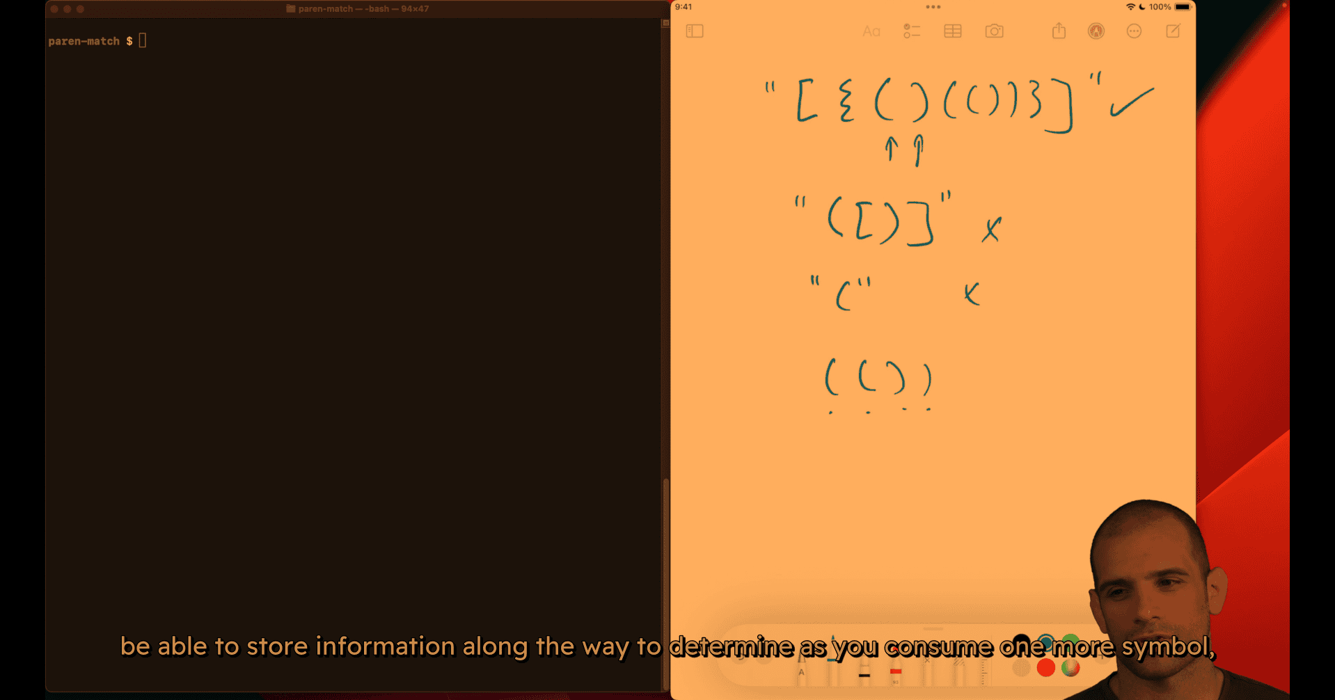
“Do I need to access things in reverse order of when I encountered them?”

If yes → Use a stack!

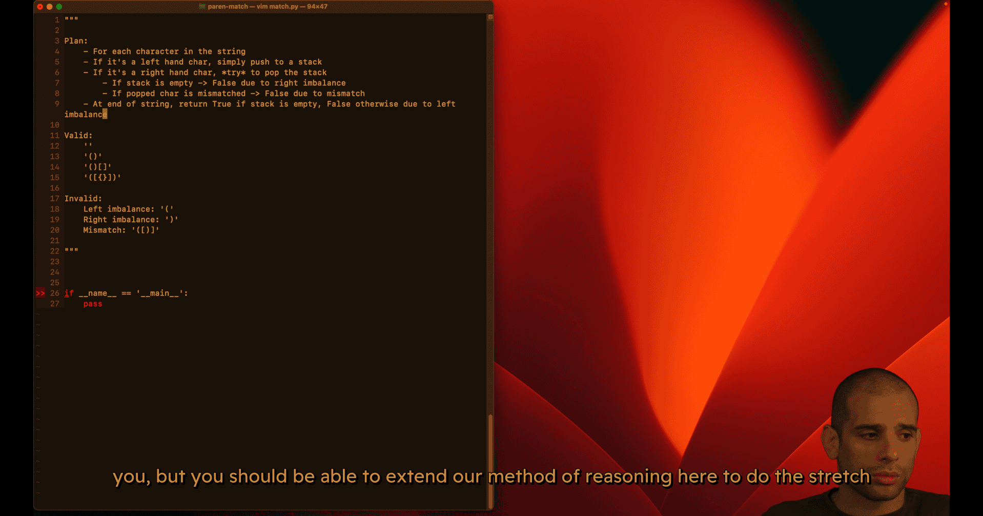
1. plan
2. small case

primer will state clear the test case , and even name the error case name ‘categorical thinking’

of the reason why this is false. I just like being categorical and having a kind of model type of error and so on in the test cases.

step1 :

step 2 :

matches left:

up in our dictionary is not equal to the new value, then we have a mismatch. Maybe actually

"""
Parenthesis Matching Implementation
Based on the algorithm plan from the lecture
"""
 
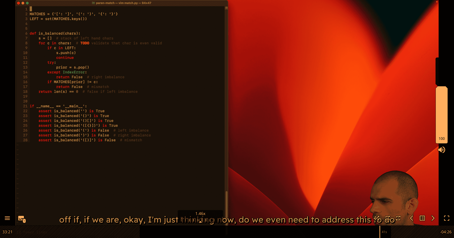
MATCHES = {'[': ']', '(': ')', '{': '}'}
LEFT = set(MATCHES.keys())
RIGHT = set(MATCHES.values())
 
def is_balanced(chars):
    """
    Plan:
    - For each character in the string
    - If it's a left hand char, simply push to a stack
    - If it's a right hand char, *try* to pop the stack
      - If stack is empty -> False due to right imbalance
      - If popped char is mismatched -> False due to mismatch
    - At end of string, return True if stack is empty, False otherwise due to left imbalance
    """
    s = []  # stack of left hand chars
    for c in chars:  # TODO: validate that char is even valid
        if c in LEFT:
            s.append(c)  # Fixed: Python lists use append(), not push()
            continue
        if c not in RIGHT: # Space case
          continue
        try:
            prior = s.pop()
        except IndexError:
            return False  # right imbalance
        if MATCHES[prior] != c:
            return False  # mismatch
    return len(s) == 0  # false if left imbalance
 
 
if __name__ == '__main__':
    # Valid cases
    assert is_balanced('') is True
    assert is_balanced('()') is True
    assert is_balanced('()[]{}') is True
    assert is_balanced('({[]})') is True
    
    # Invalid cases
    assert is_balanced('(') is False  # left imbalance
    assert is_balanced(')') is False  # right imbalance
    assert is_balanced('([)]') is False  # mismatch
    
    print("All tests passed!")
 

---

016 Doubly linked list.mp4

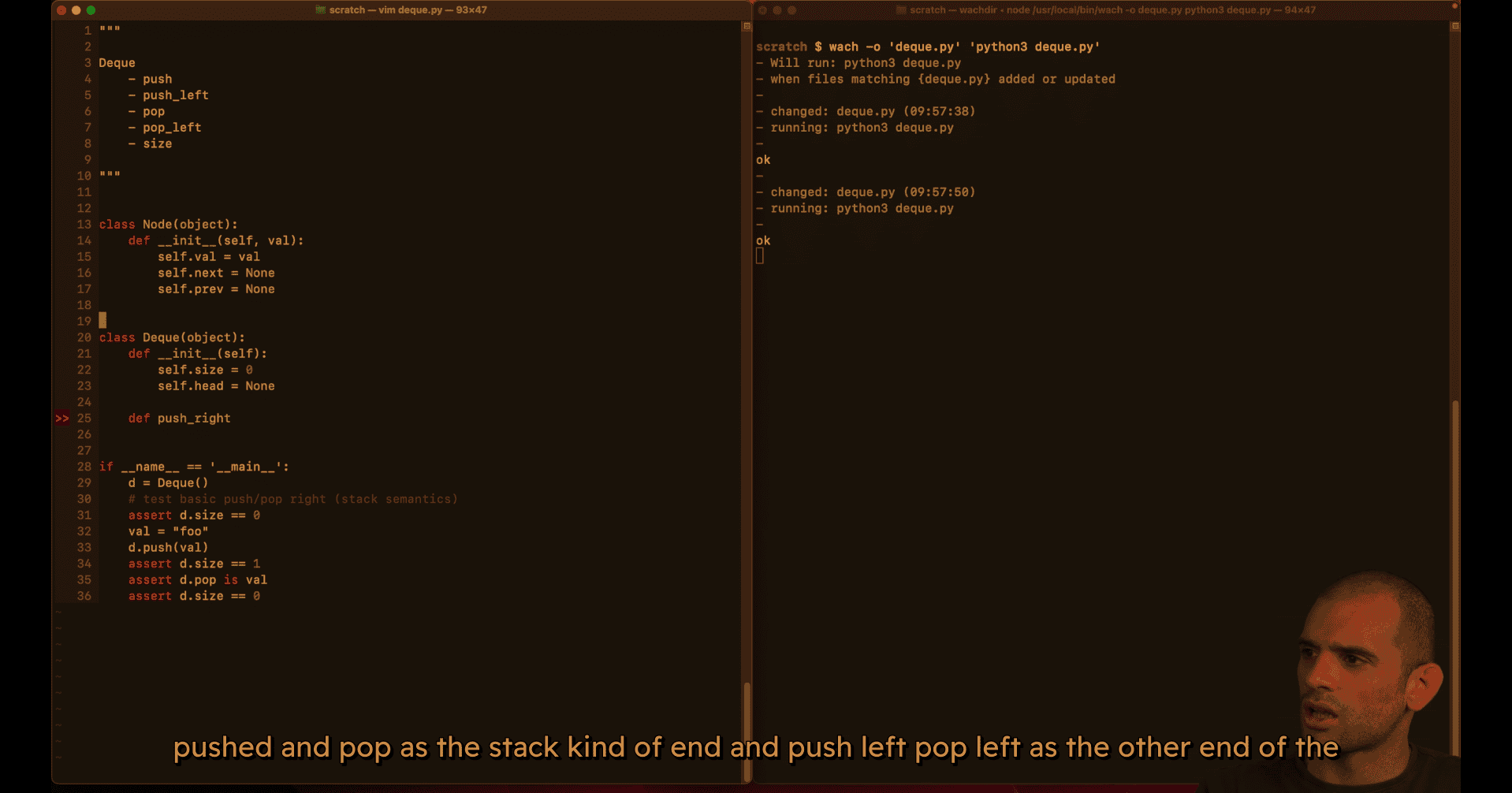
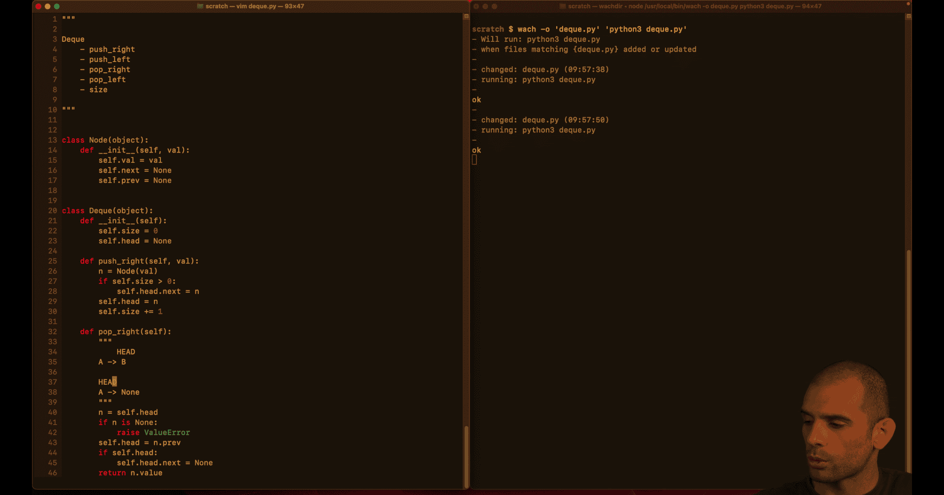
using comment to show the mvp e.g.

double linked list: head become tail, next become prev

1. empty case

/home/peter/Desktop/cursor_project/doubly-linked-list-notes.md

Memory Management: Critical Considerations

The Problem: Circular References

Circular reference example:

## Node A points to Node B
A.next = B
B.prev = A
 
## Even if nothing else references A or B,
## they still reference each other!
## Reference count never drops to zero

In Python:

• Reference counting: Fast, but fails with circular references
• Tracing garbage collection: Slow, but handles circular references
• Best practice: Break references explicitly to avoid circular references

Solution: Always Break Links

When removing a node:

1. Set next = None on the node before it
2. Set prev = None on the node after it
3. Update head/tail appropriately
4. Set head/tail to None when deque becomes empty

Example in pop_right:

self.head = n.prev        # Move head back
if self.head is not None:
    self.head.next = None  # Break forward link (critical!)
else:
    self.tail = None       # Also clear tail if empty

Why This Matters

Long-running processes:

• Servers, databases, web applications
• Memory leaks accumulate over time
• Can cause performance degradation or crashes

Best practice:

• Always set pointers to None when removing nodes
• Be explicit about breaking references
• Test that memory is properly reclaimed

---

017 Basic calculator.mp4

plan :

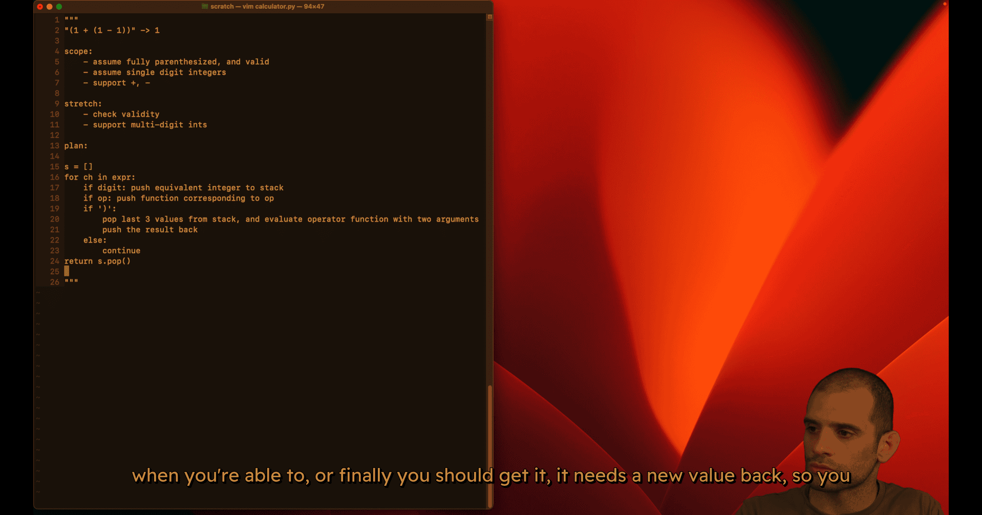
test case:

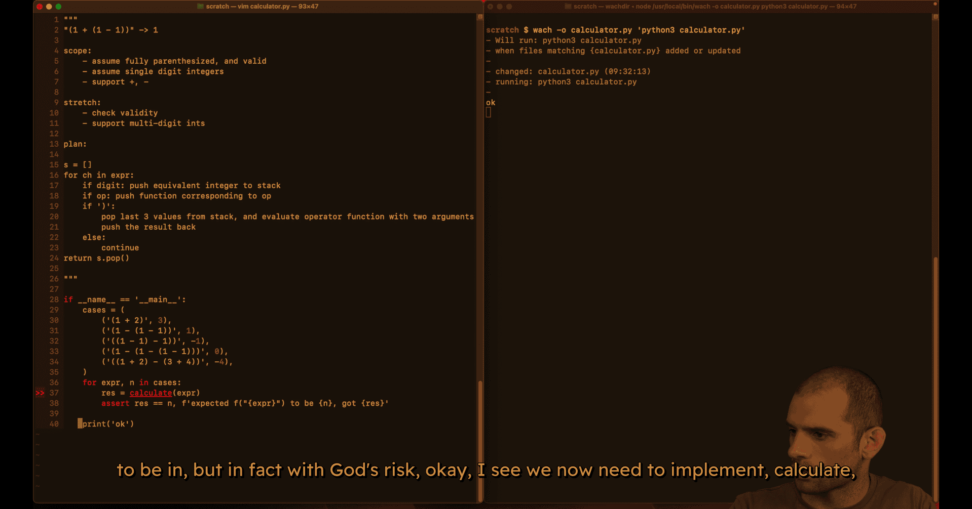
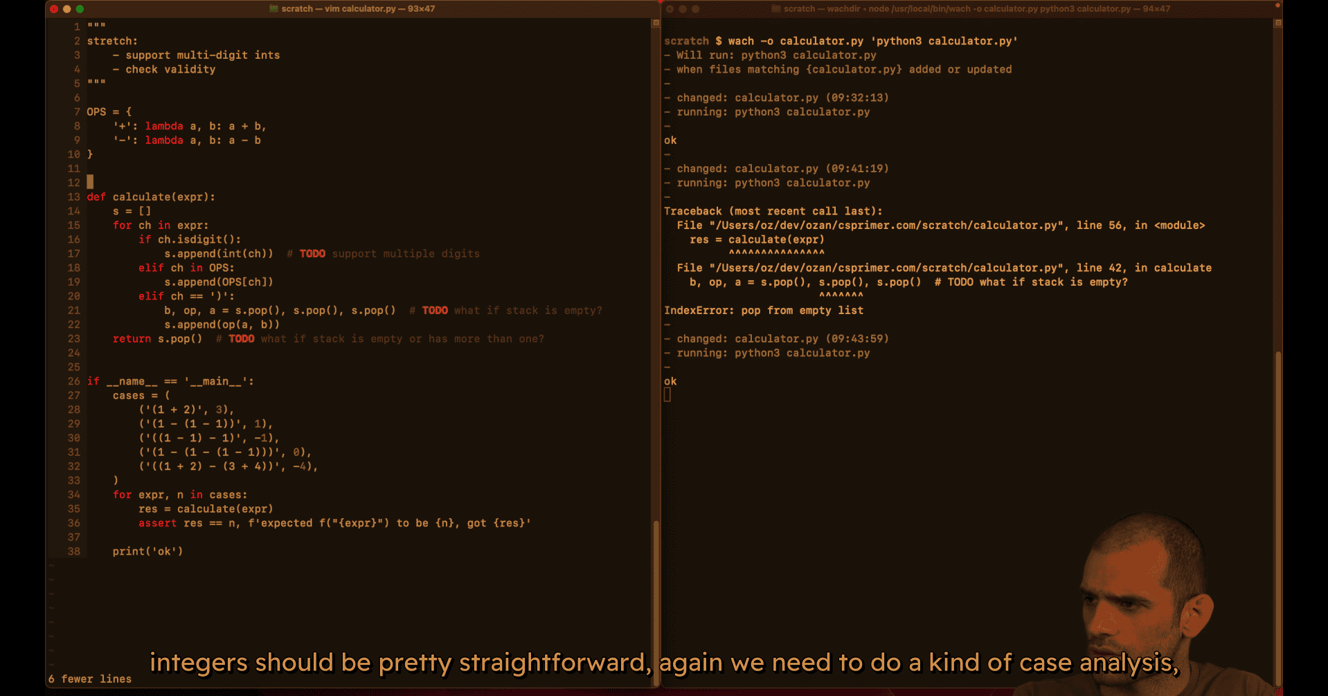
mvp (single digit mode work)

primer logic for double digit :

if len(is) == 0 or not isinstance(s[-i],int):
  s.append(int(ch))
else:
  s[-1]=s[-1]*10+int(ch)

gpt logic:

            # Combine with previous digit if present (multi-digit support)
            if stack and isinstance(stack[-1], int):
                stack[-1] = stack[-1] * 10 + digit
            else:
                stack.append(digit)