cs61a-part2
cs61a COMPOSING PROGRAMS CS 61A Spring 2025 question: Cats | CS自学社区 ans: [2021 Spring] CS61A 学习笔记 索引 - ikventure - 博客园 - quite good ans
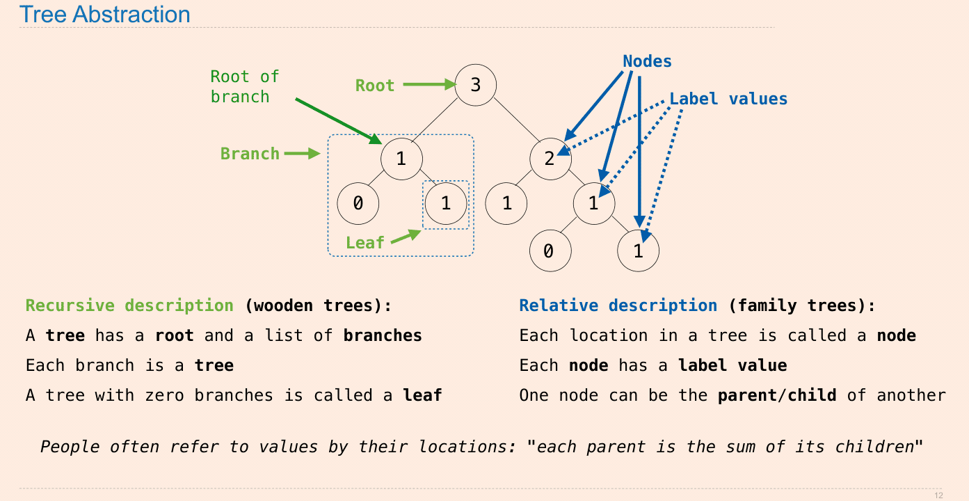
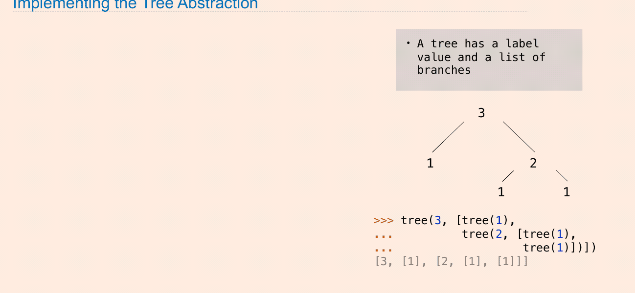
Tree
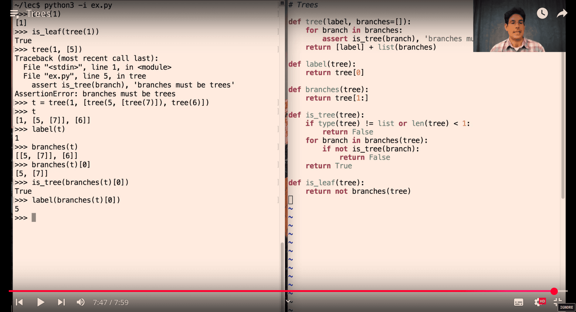
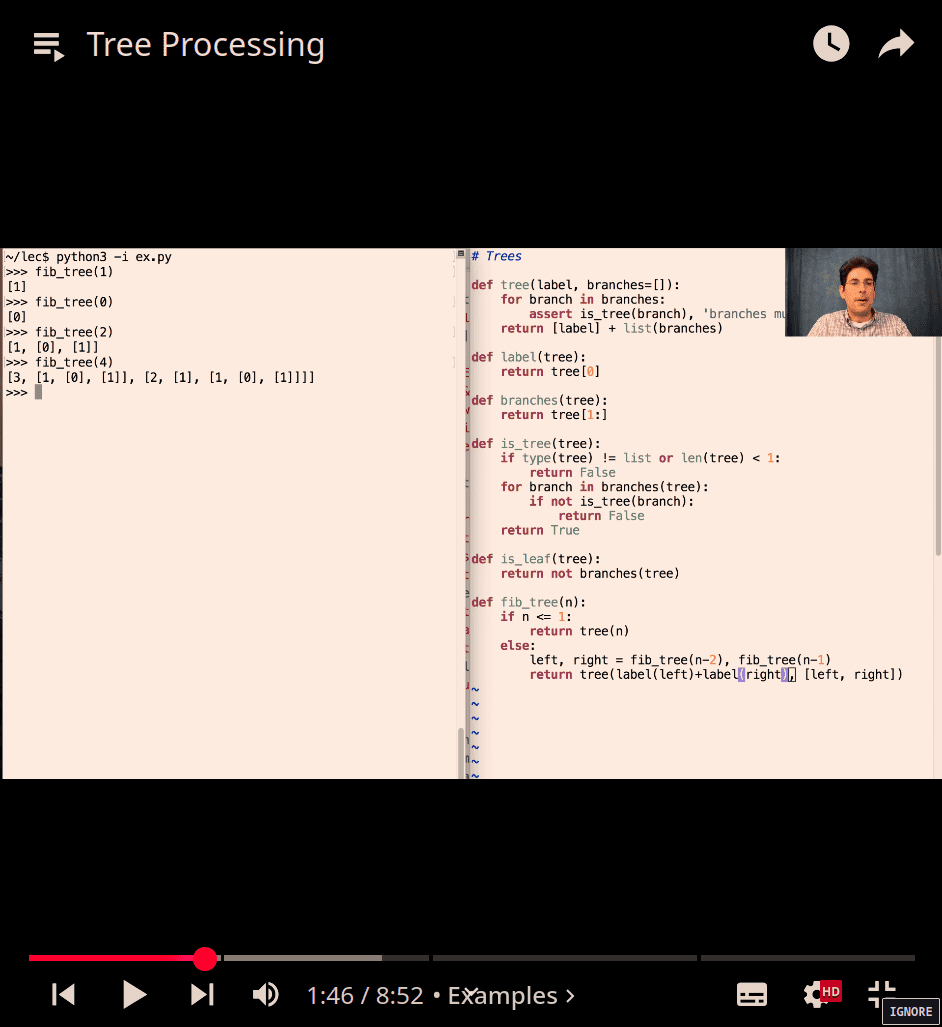
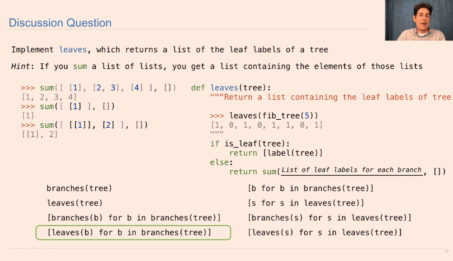
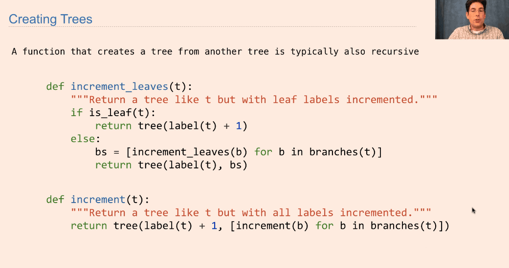
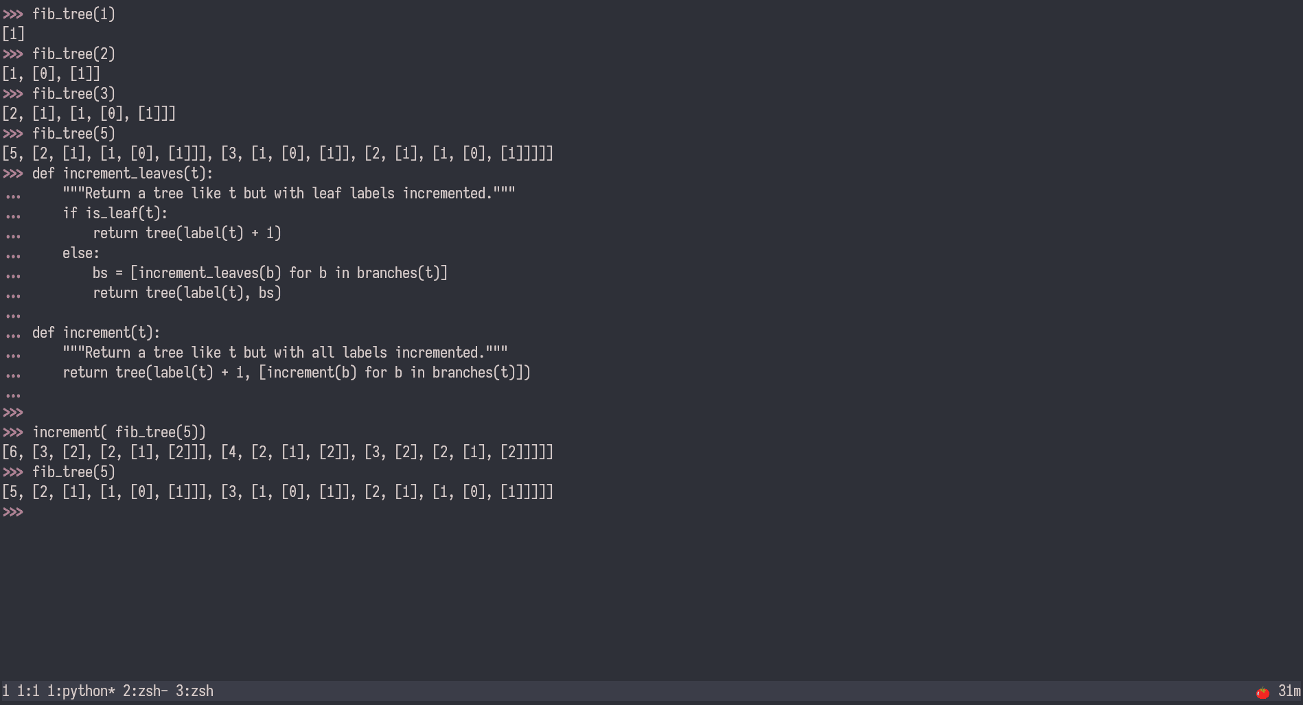
- it add 1 to all the node including the lable

- increment the leaves only
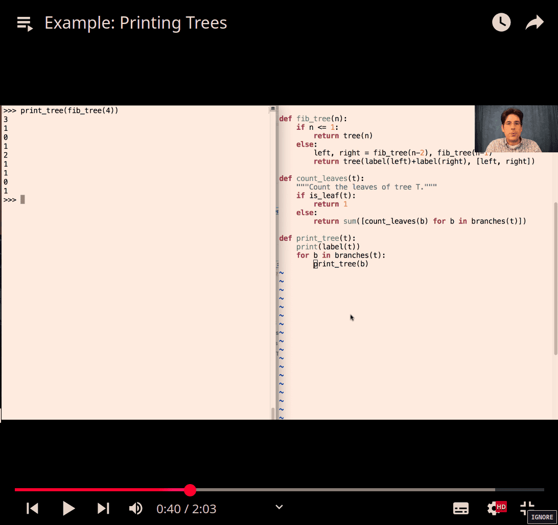
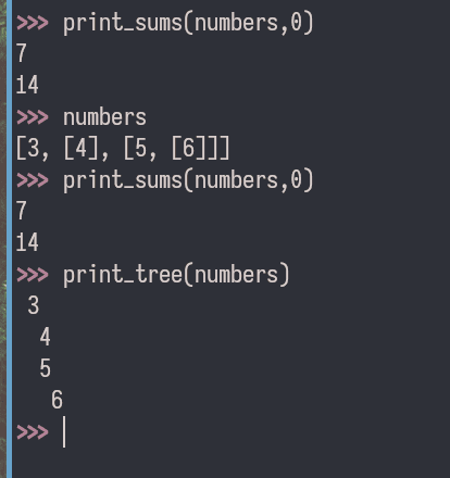
first print tree
def print_tree(t, indent=0):
    print(' '*indent, label(t)) # could adding str() to label
    for b in branches(t):
print_tree(b, indent + 1)- fib_tree make it much easier to see the difference

numbers = tree(3, [tree(4), tree(5, [tree(6)])])
haste = tree('h', [tree('a', [tree('s'),
                              tree('t')]),
                   tree('e')])

>>> haste
['h', ['a', ['s'], ['t']], ['e']]
>>> print_tree(haste)
 h
  a
   s
   t
  e
  >>> label(haste)
  'h'
  >>> branches(haste)
  [['a', ['s'], ['t']], ['e']]
- adding a function
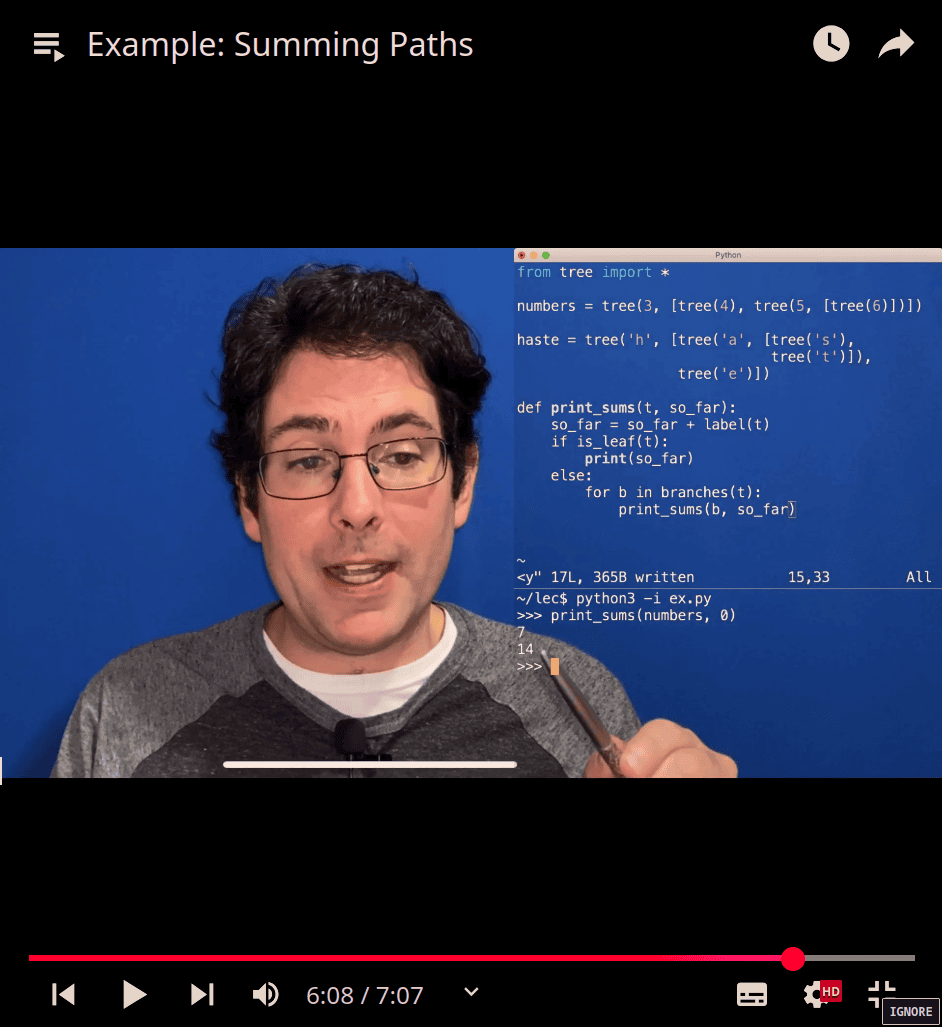
def print_sums(t, so_far):
    so_far = so_far + label(t)
    if is_leaf(t):
        print(so_far)
    else:
        for b in branches(t):
            print_sums(b, so_far)
  >>> numbers
  [3, [4], [5, [6]]]
  >>> print_sums(numbers,0)
  7
  14
  >>>
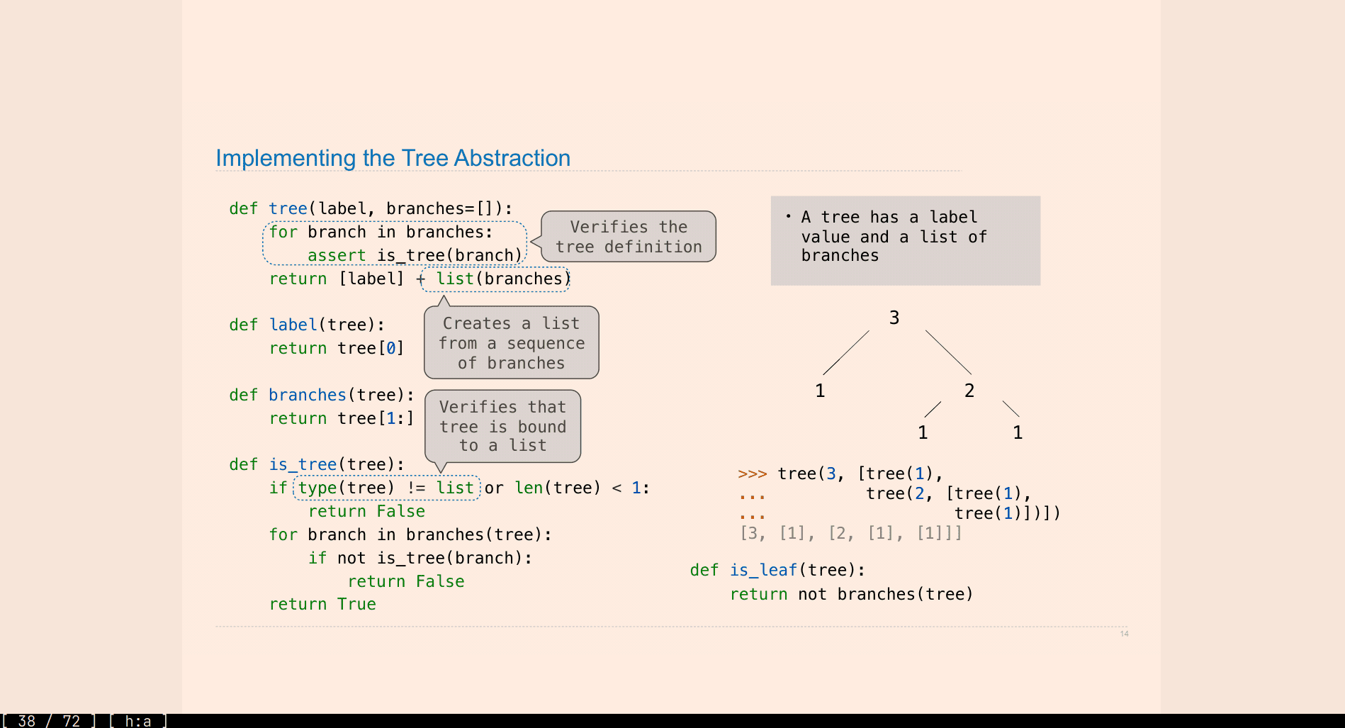
The expression not branches(list) will return:
True→ whenbranches(list)is an empty list ([]), meaninglisthas no branches (only a root).False→ whenbranches(list)is not empty, meaninglisthas at least one branch.
Example Scenarios:
tree1 = [1]          # Only root, no branches
tree2 = [1, [2], [3]]  # Root with branches

print(not branches(tree1))  # True (empty branches)
print(not branches(tree2))  # False (has branches)
So, is_leaf(tree) will return True only when the tree has no branches.
- empty list → false (TF game)
>>> print_sums(numbers,0)
7
14
>>> numbers
[3, [4], [5, [6]]]
>>> print_sums(numbers,0)
7
14
>>> print_tree(numbers)
 3
  4
  5
   6
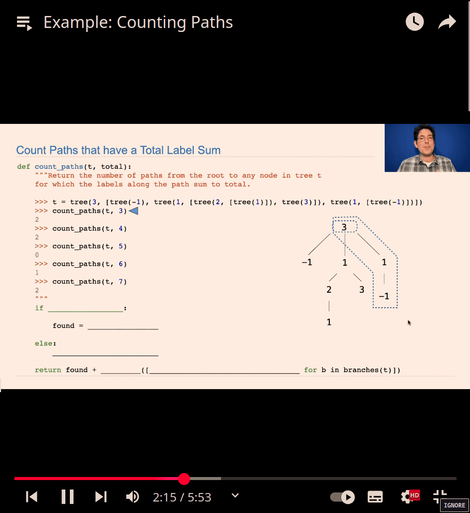
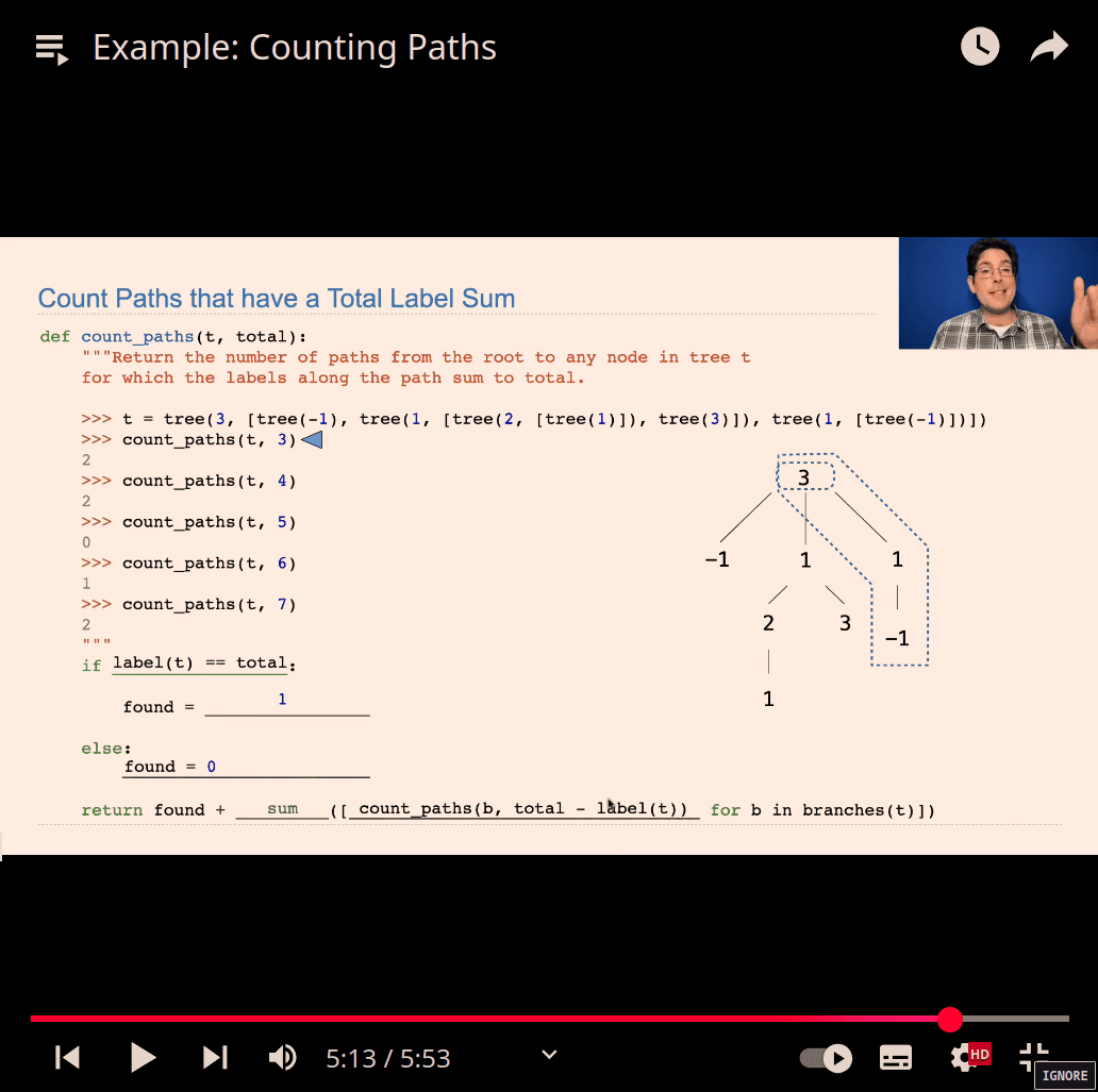
find total path to get the number total
- how many way to get the ans
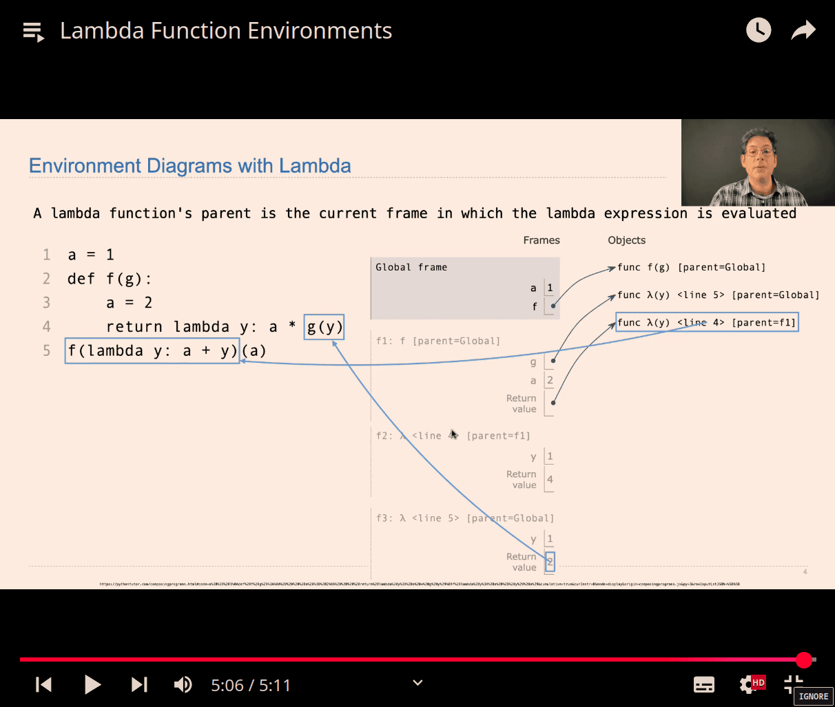
- review :→
(a) → variable → 1
second(thing ) into a fuction: → into return (y)
a → y , so y = 1
g() call back parent fuction (a / 1)
lambda y:
>>> a = 3
...
... def f(g):
...     a = 2
...     return lambda y: a* g(y)
... f(lambda y : a+y )(a)
...
12
>>>

(a) -> into another (variable)

  - indent -> trace
  last step is *2
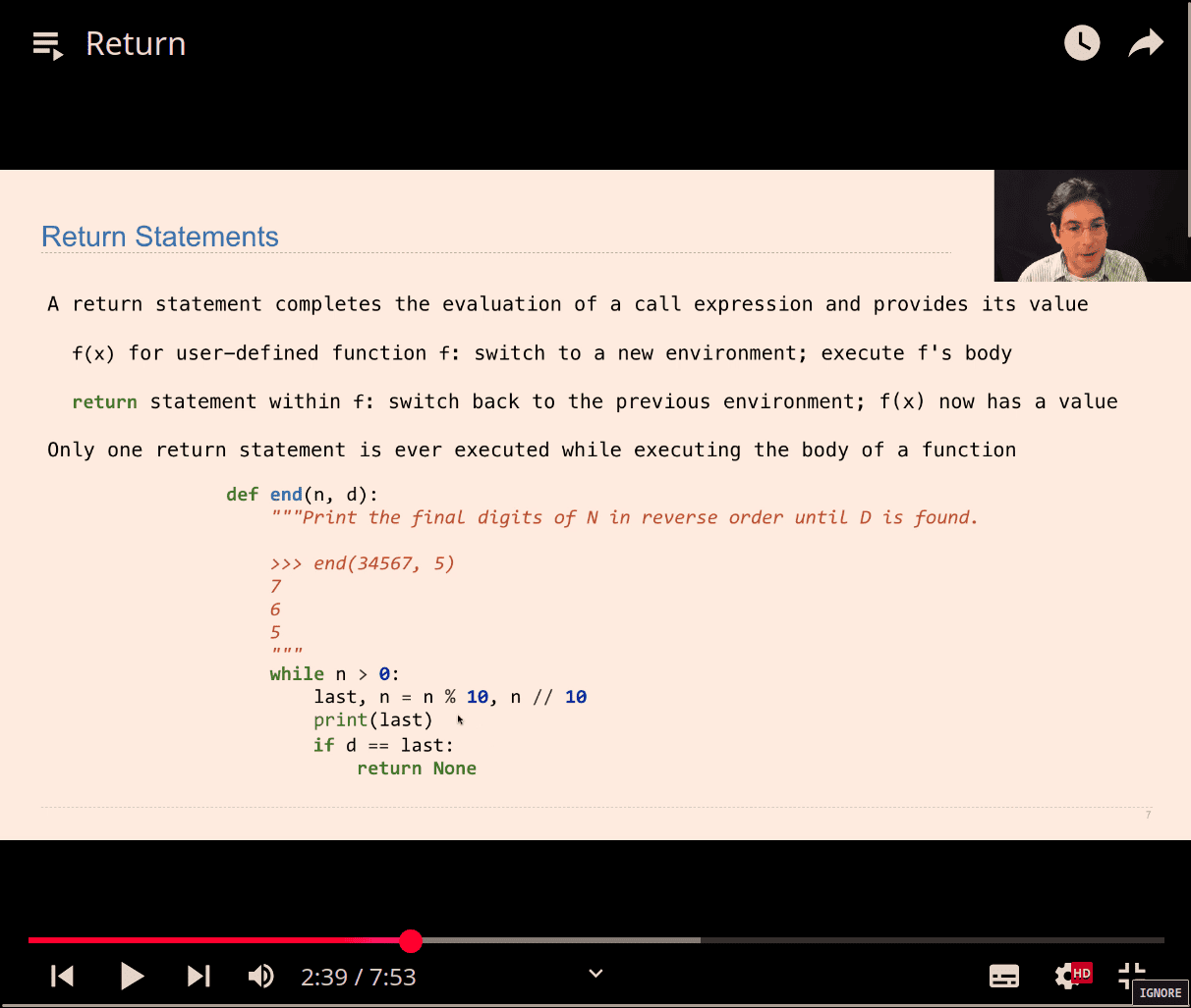
- return None → ending the fuction
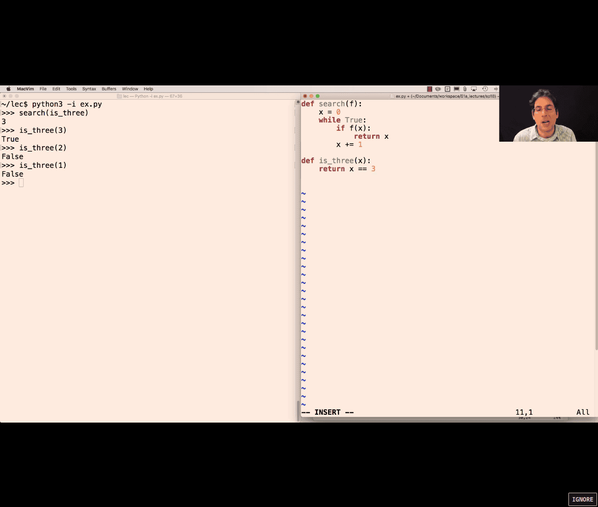
- brute force
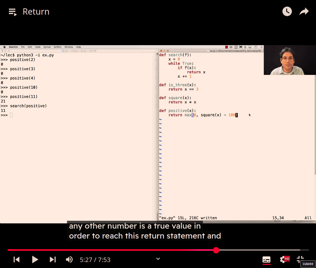
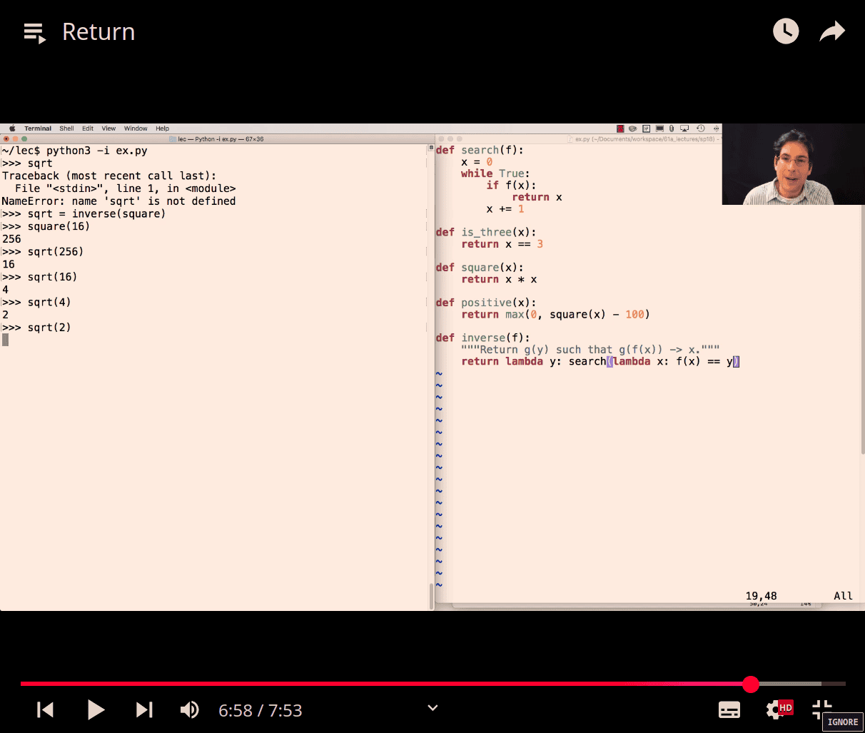
y = last ( variable )
search (f) → anyfn that f(self) = y , if true = return x
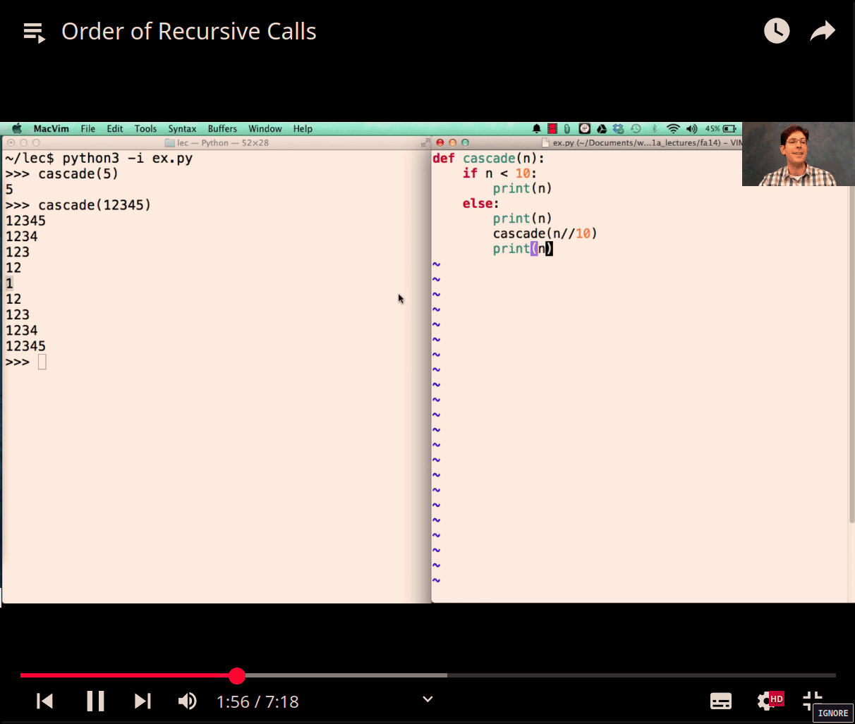
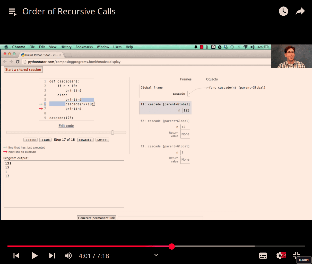
- return None make a back to previous recurion fn 🤔
- damn , so that’s why it print both case !!!!
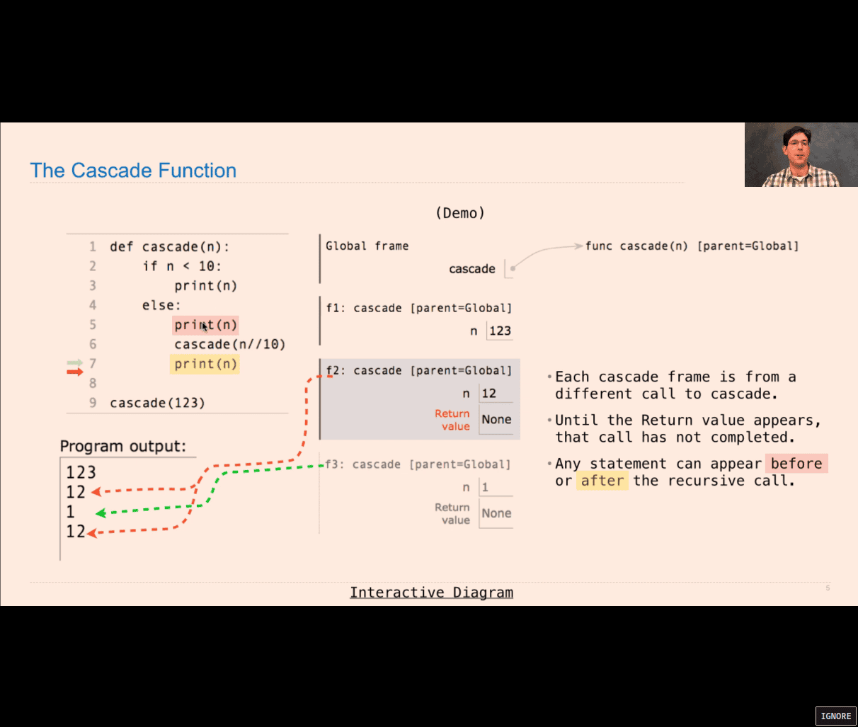
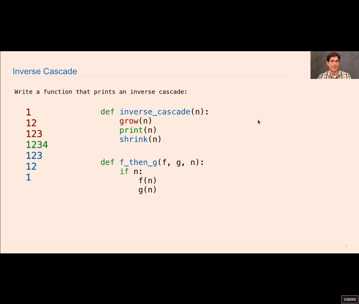
<Each cascade frame is from a different call to cascade.
-Until the Return value appears, that call has not completed.
«Any statement can appear before or after the recursive call.
shorter version:
def cascade(n):
    print(n)
    if n>10:
        cascade(n//10)
        print(n)
longer implemenation is more clear (base case, recursive case , so first one is better)
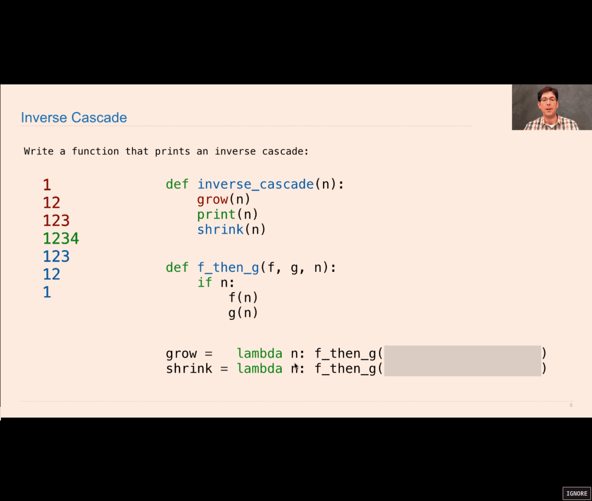
now it is inverse cascade:
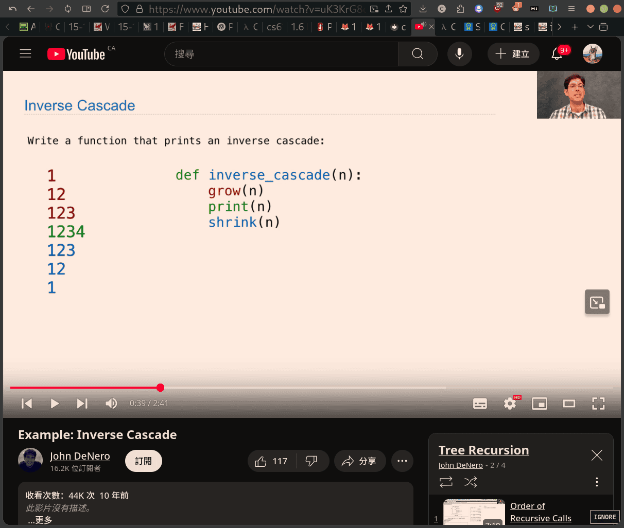

- Tree recursion
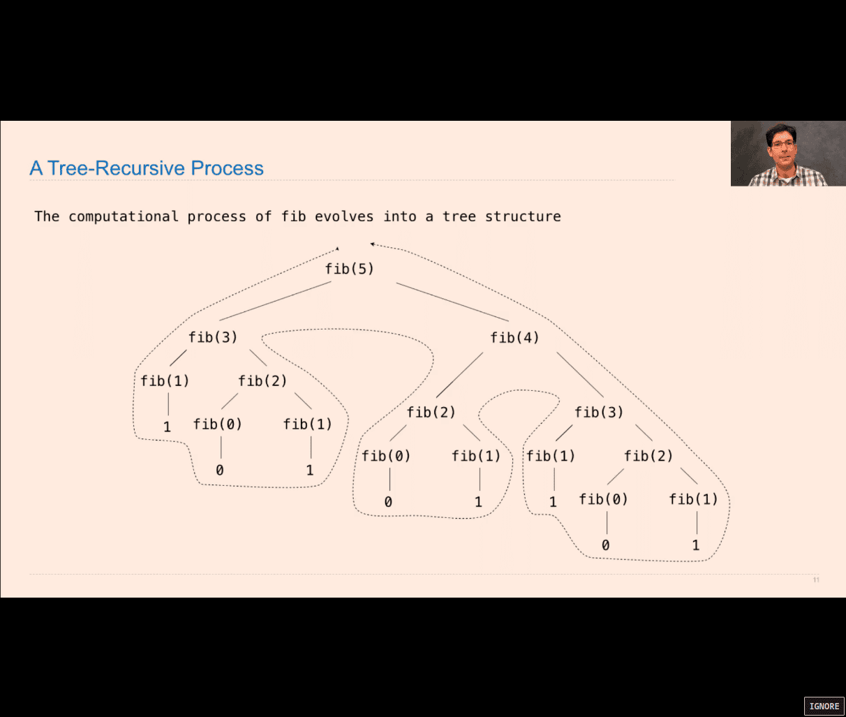
>>> fib(0)
0
>>> fib(1)
1
>>> fib(3)
2
>>> fib(5)
5
>>> fib(6)
8
>>> fib(8)
21
>>>
  @trace
def fib(n):
    if n == 0:
        return 0
    elif n == 1:
        return 1
    else:
        return fib(n - 2) + fib(n - 1)
- using ucb trace.py to trace the recursion function 🤩🤩🤩
ucb python file:
"""The UCB module contains functions specific to 61A projects at UC Berkeley."""

import code
import functools
import inspect
import re
import signal
import sys


def main(fn):
    """Call fn with command line arguments.  Used as a decorator.

    The main decorator marks the function that starts a program. For example,

    @main
    def my_run_function():
        # function body

    Use this instead of the typical __name__ == "__main__" predicate.
    """
    if inspect.stack()[1][0].f_locals['__name__'] == '__main__':
        args = sys.argv[1:] # Discard the script name from command line
        fn(*args) # Call the main function
    return fn

_PREFIX = ''
def trace(fn):
    """A decorator that prints a function's name, its arguments, and its return
    values each time the function is called. For example,

    @trace
    def compute_something(x, y):
        # function body
    """
    @functools.wraps(fn)
    def wrapped(*args, **kwds):
        global _PREFIX
        reprs = [repr(e) for e in args]
        reprs += [repr(k) + '=' + repr(v) for k, v in kwds.items()]
        log('{0}({1})'.format(fn.__name__, ', '.join(reprs)) + ':')
        _PREFIX += '    '
        try:
            result = fn(*args, **kwds)
            _PREFIX = _PREFIX[:-4]
        except Exception as e:
            log(fn.__name__ + ' exited via exception')
            _PREFIX = _PREFIX[:-4]
            raise
        # Here, print out the return value.
        log('{0}({1}) -> {2}'.format(fn.__name__, ', '.join(reprs), result))
        return result
    return wrapped


def log(message):
    """Print an indented message (used with trace)."""
    print(_PREFIX + re.sub('\n', '\n' + _PREFIX, str(message)))


def log_current_line():
    """Print information about the current line of code."""
    frame = inspect.stack()[1]
    log('Current line: File "{f[1]}", line {f[2]}, in {f[3]}'.format(f=frame))


def interact(msg=None):
    """Start an interactive interpreter session in the current environment.

    On Unix:
      <Control>-D exits the interactive session and returns to normal execution.
    In Windows:
      <Control>-Z <Enter> exits the interactive session and returns to normal
      execution.
    """
    # evaluate commands in current namespace
    frame = inspect.currentframe().f_back
    namespace = frame.f_globals.copy()
    namespace.update(frame.f_locals)

    # exit on interrupt
    def handler(signum, frame):
        print()
        exit(0)
    signal.signal(signal.SIGINT, handler)

    if not msg:
        _, filename, line, _, _, _ = inspect.stack()[1]
        msg = 'Interacting at File "{0}", line {1} \n'.format(filename, line)
        msg += '    Unix:    <Control>-D continues the program; \n'
        msg += '    Windows: <Control>-Z <Enter> continues the program; \n'
        msg += '    exit() or <Control>-C exits the program'

code.interact(msg, None, namespace)- with trace(ubc)
>>> fib(0)
fib(0):
fib(0) -> 0
0
>>> fib(1)
fib(1):
fib(1) -> 1
1
>>> fib(2)
fib(2):
    fib(0):
    fib(0) -> 0
    fib(1):
    fib(1) -> 1
fib(2) -> 1
1
>>> fib(3)
fib(3):
    fib(1):
    fib(1) -> 1
    fib(2):
        fib(0):
        fib(0) -> 0
        fib(1):
        fib(1) -> 1
    fib(2) -> 1
fib(3) -> 2
2
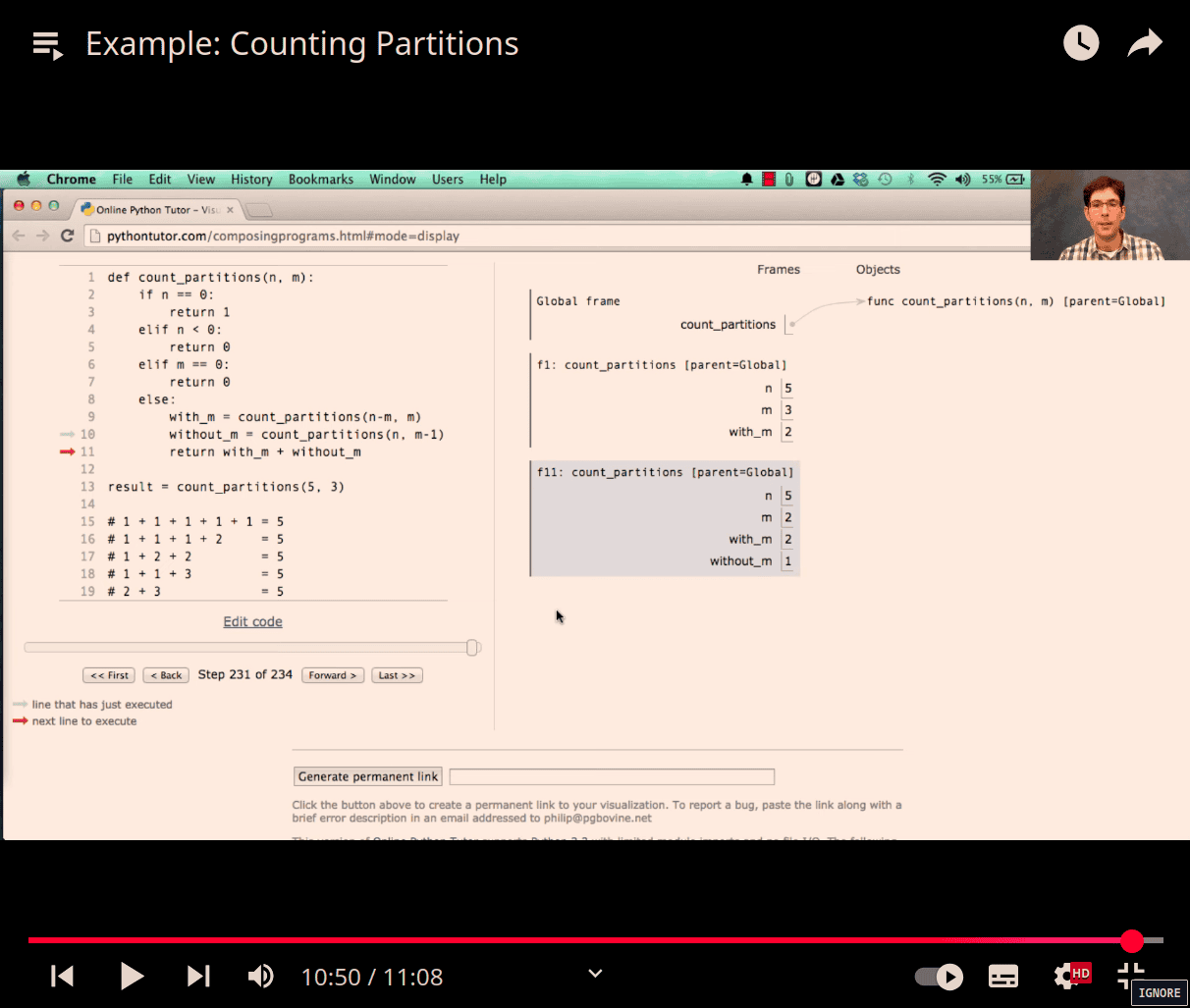
- tree partitions
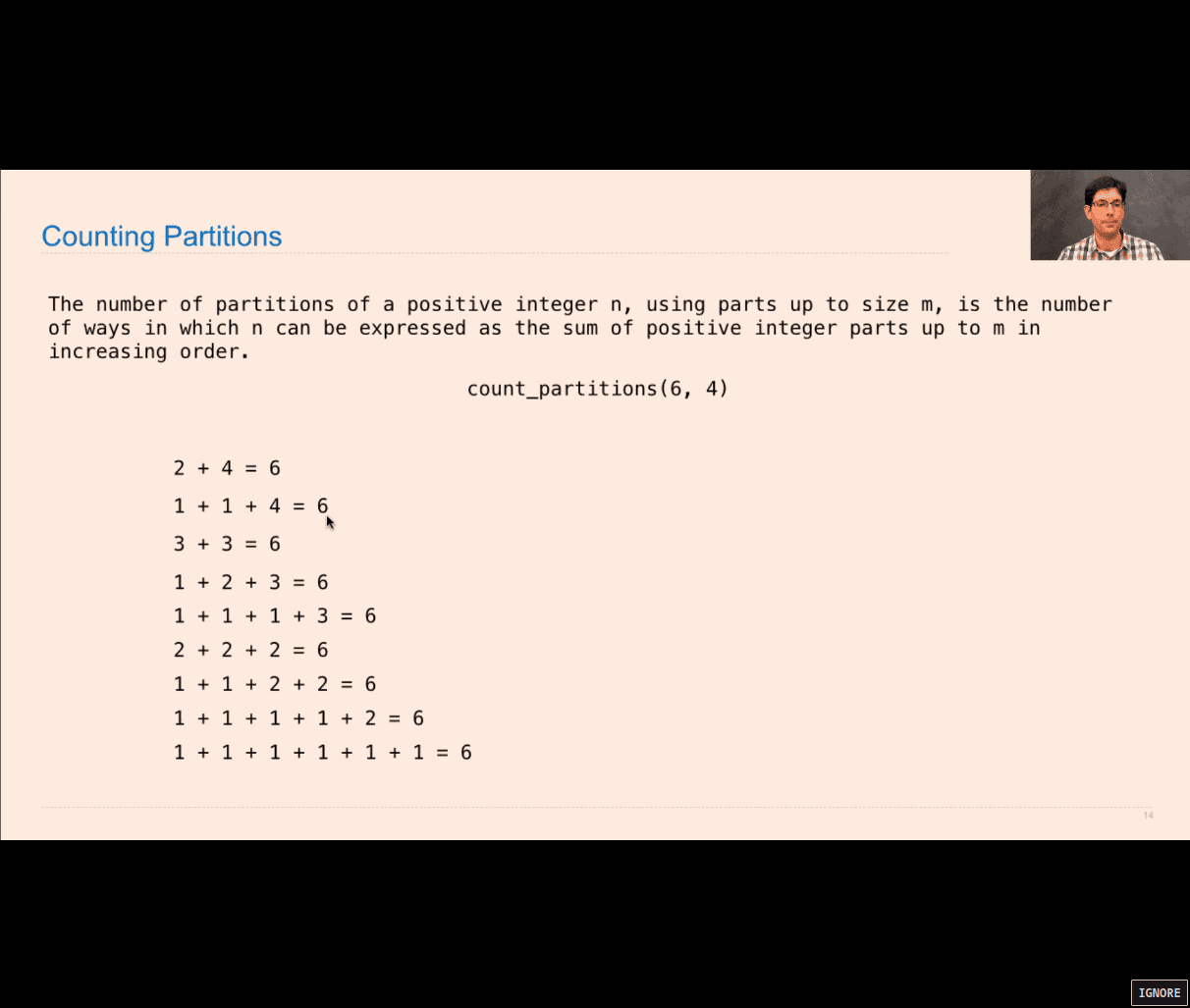
- counting 6, but max for using number 4
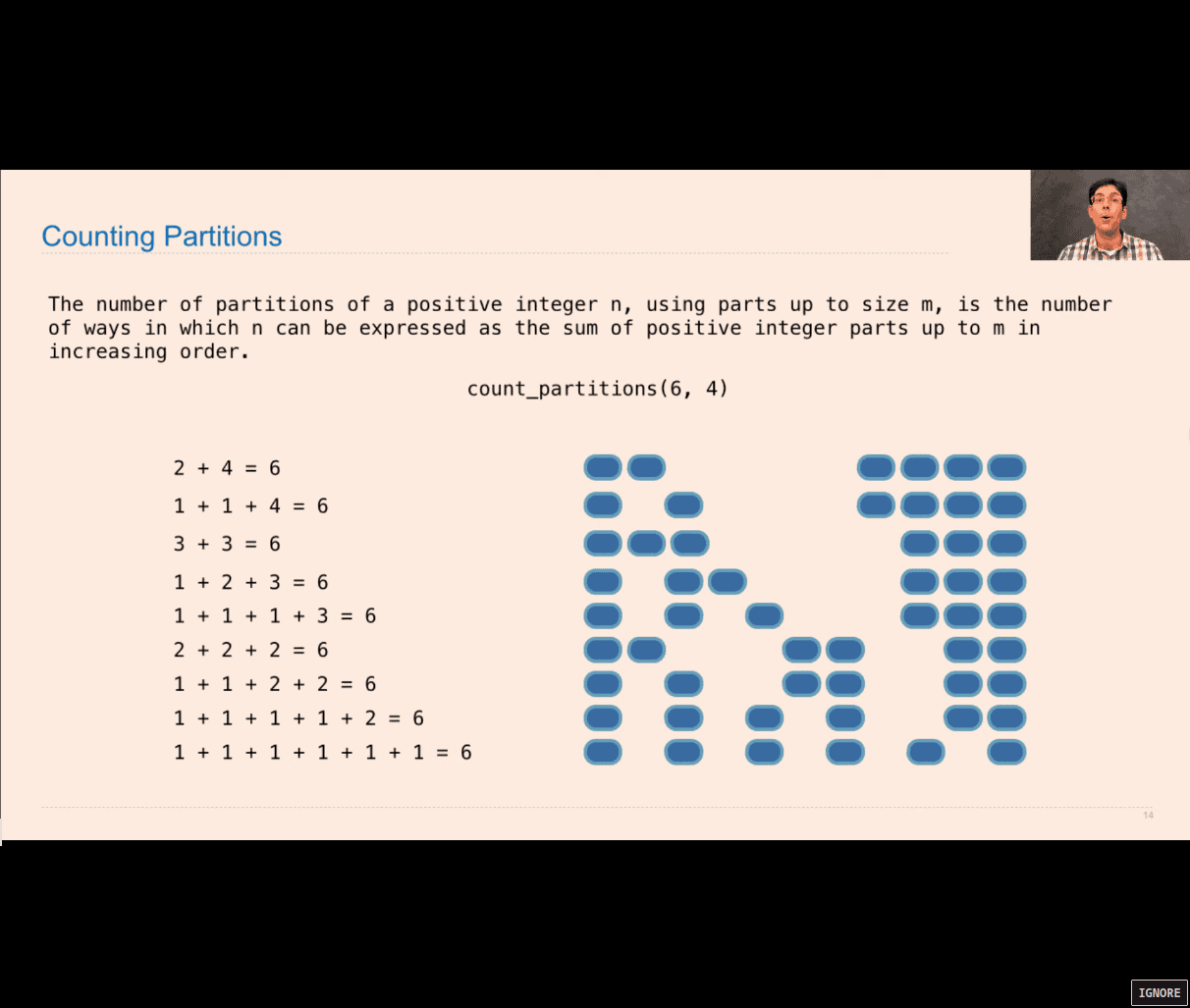
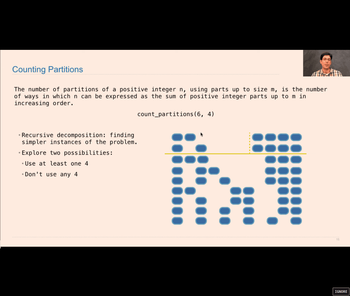
- spliting half
left = 6-4
right =
explore two possibilities:
- use at least one 4
- don’t use any 4
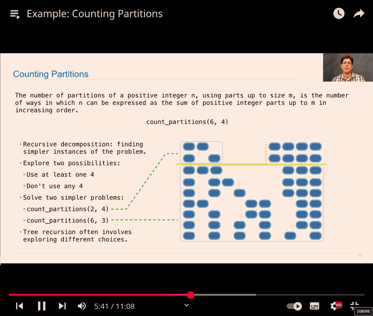
Decomposing problem
-
count_partitions(2, 4)
-
count_partitions(6, 3)
again , at least 3 , don’t use 3
finally , sum them all
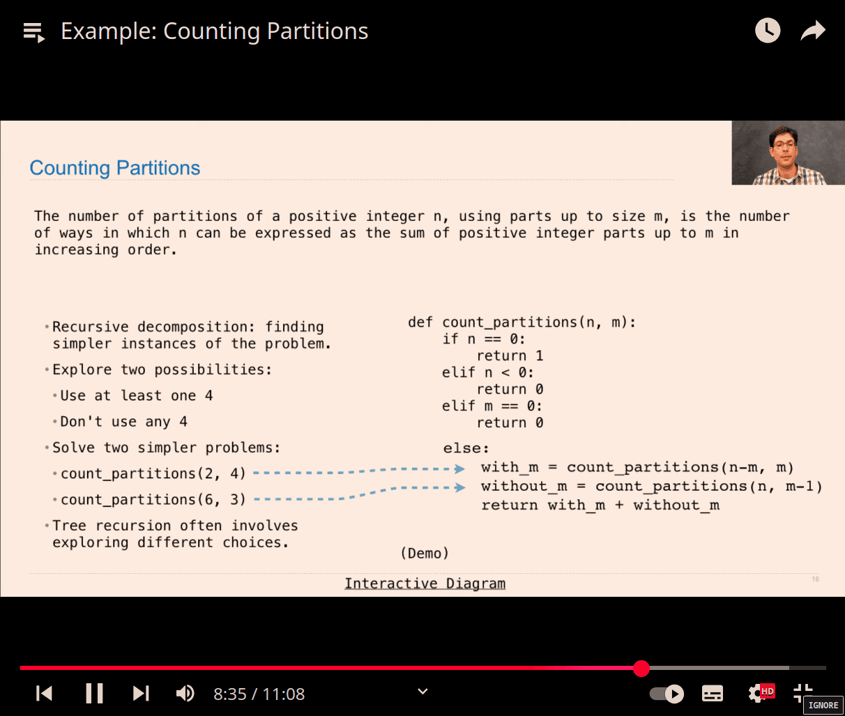
@trace
def count_partitions(n, m):
    if n == 0:
        return 1
    elif n < 0:
        return 0
    elif m == 0:
        return 0
    else:
        with_m = count_partitions(n - m, m)
        without_m = count_partitions(n, m - 1)
        return with_m + without_m

>>> count_partitions(2,4)
count_partitions(2, 4):
    count_partitions(-2, 4):
    count_partitions(-2, 4) -> 0
    count_partitions(2, 3):
        count_partitions(-1, 3):
        count_partitions(-1, 3) -> 0
        count_partitions(2, 2):
            count_partitions(0, 2):
            count_partitions(0, 2) -> 1
            count_partitions(2, 1):
                count_partitions(1, 1):
                    count_partitions(0, 1):
                    count_partitions(0, 1) -> 1
                    count_partitions(1, 0):
                    count_partitions(1, 0) -> 0
                count_partitions(1, 1) -> 1
                count_partitions(2, 0):
                count_partitions(2, 0) -> 0
            count_partitions(2, 1) -> 1
        count_partitions(2, 2) -> 2
    count_partitions(2, 3) -> 2
count_partitions(2, 4) -> 2
2
(4,6)
1.  6 = 2 + 4
2.  6 = 1 + 1 + 4
3.  6 = 3 + 3
4.  6 = 1 + 2 + 3
5.  6 = 1 + 1 + 1 + 3
6.  6 = 2 + 2 + 2
7.  6 = 1 + 1 + 2 + 2
8.  6 = 1 + 1 + 1 + 1 + 2
9.  6 = 1 + 1 + 1 + 1 + 1 + 1
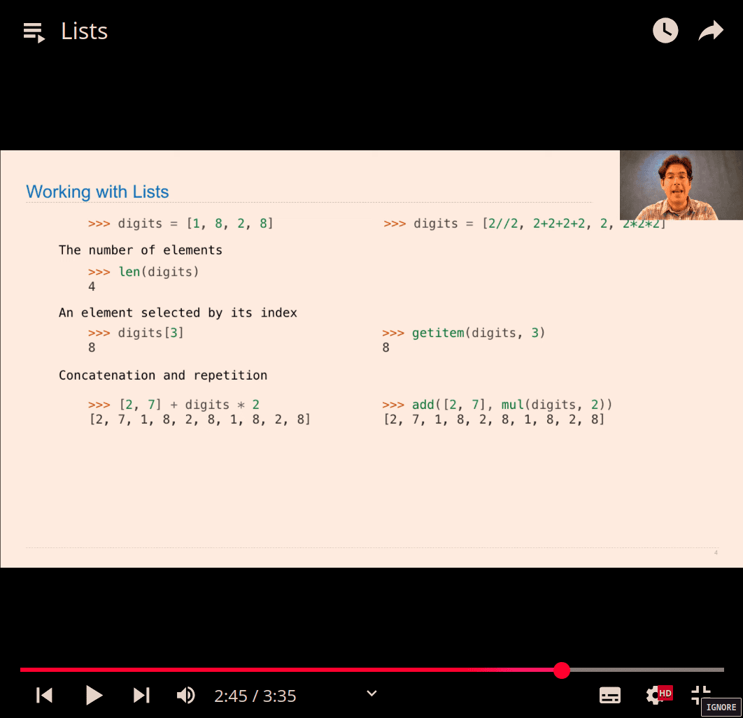
digit[3] or getitem(digits, 3) → same
- containers
>>> digits=[1,8,2,8]
>>> 1 in digits
True
>>> 2 in digits
True
>>> 5 not in digits
True
>>> not(5 in digits)
True
>>> '1' == 1
False
>>> '1' in digits
False
>>> [1,8] in digits
False
>>> [1,2] in [3,[1,2],4]
True
>>> [1,2] in [3,[[1,2]],4]
False
>>>
- statements
>>> def count(s, value):
...     total,index=0,0
...     while index<len(s):
...         element=s[index]
...         if element == value:
...             total = total +1
...         index=index+1
...     return total
...
>>> count([1,2,1,2,1],1)
3
# refactor into python prefer:
def count_new(s, value):
    total = 0
    for element in s:
        if element == value:
            total += 1
    return total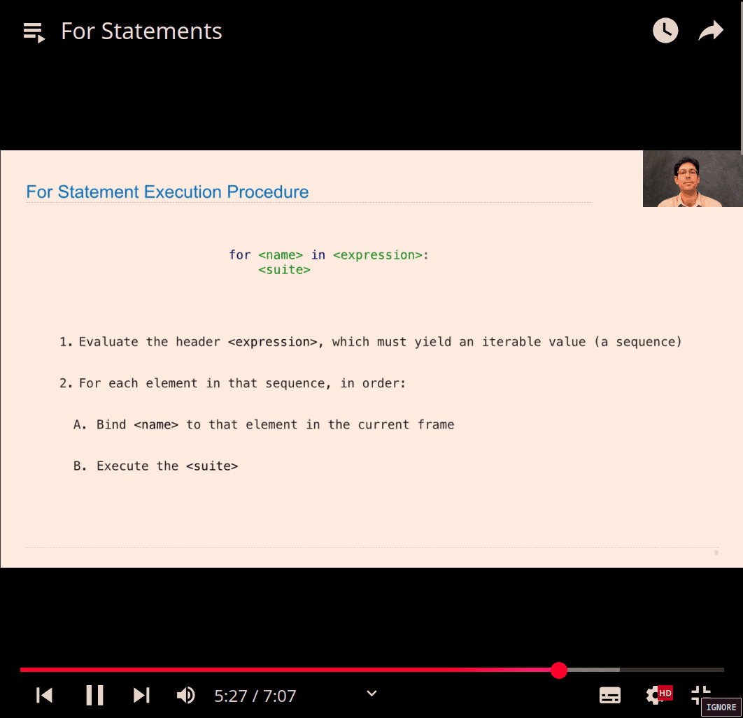
-
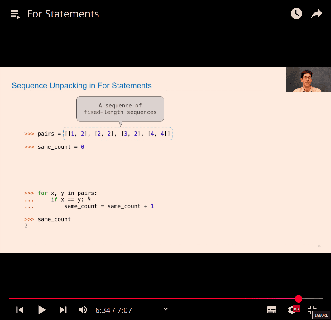
unpack the pairs (only work in same length sequence) for x,y in pairs: if x==y:
-
range:
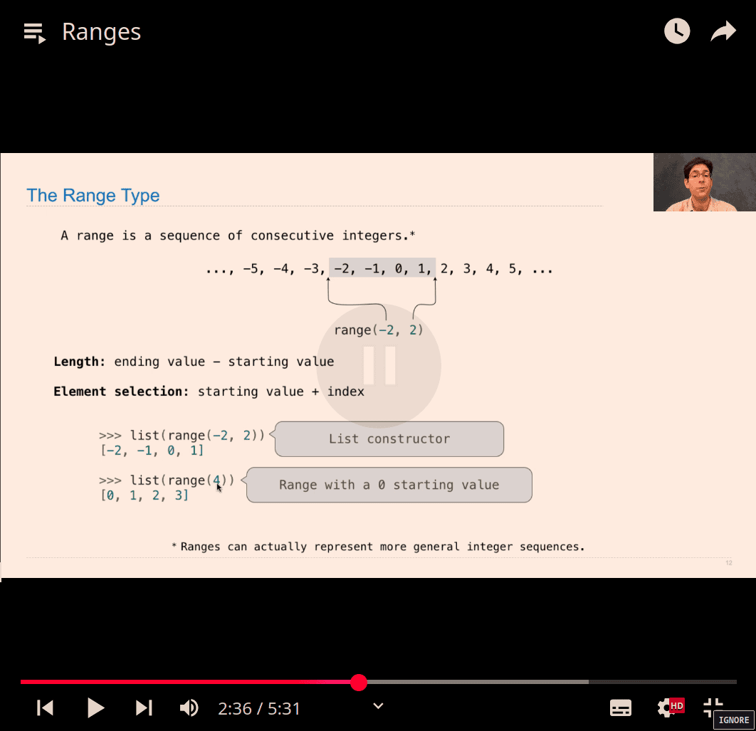
- list(range())
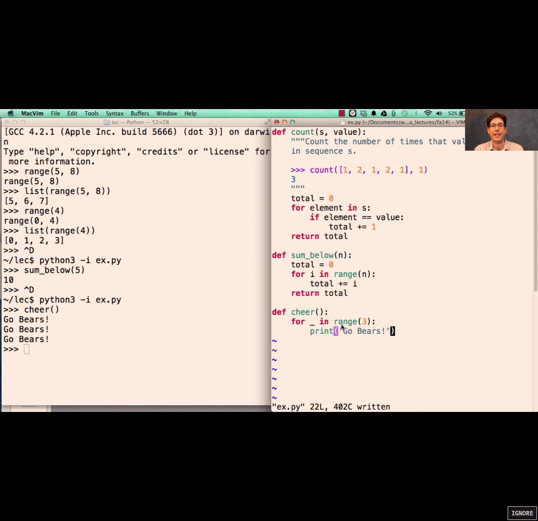
for _ in range(3):
- just loop 3 time
- list comprehensions
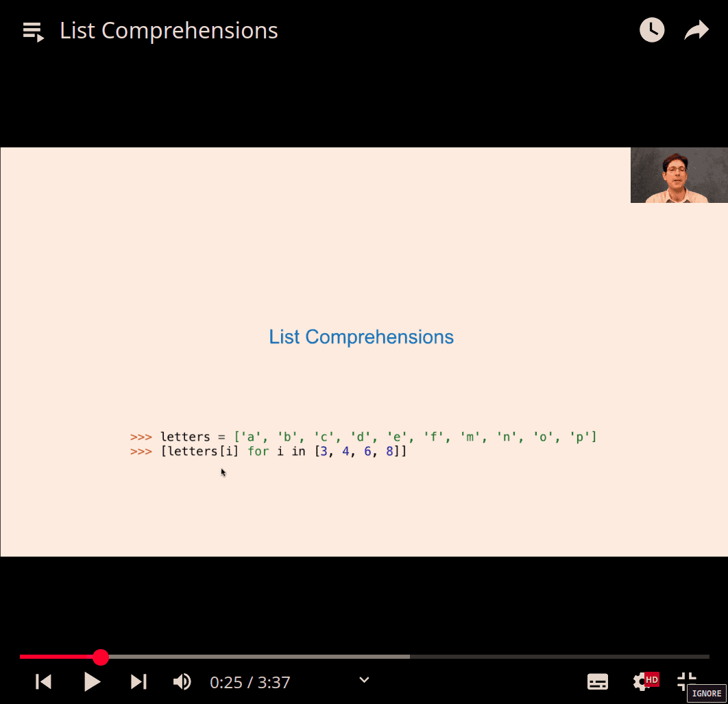
>>> odds =[1,3,5,7,9]
>>> [x+1 ofr x in odds]
  File "<python-input-64>", line 1
    [x+1 ofr x in odds]
     ^^^^^^^
SyntaxError: invalid syntax. Perhaps you forgot a comma?
>>> [x+1 for x in odds]
[2, 4, 6, 8, 10]
>>> [x+2 for x in odds]
[3, 5, 7, 9, 11]
>>> [x**2 for x in odds]
[1, 9, 25, 49, 81]
>>> x**2 for x in odds
  File "<python-input-68>", line 1
    x**2 for x in odds
         ^^^
SyntaxError: invalid syntax
>>> [x**2 for x in odds]
[1, 9, 25, 49, 81]
>>> (x**2 for x in odds)
<generator object <genexpr> at 0x7a5e2cddcd40>
>>> list((x**2 for x in odds))
[1, 9, 25, 49, 81]
>>> list(x**2 for x in odds)
[1, 9, 25, 49, 81]
>>> [x**2 for x in list(x**2 for x in odds)]
[1, 81, 625, 2401, 6561]
>>> [x for x in odds if 25 %x ==0]
[1, 5]

## other list compre:
>>> def divisor(n):
...     return [1] + [x for x in range(2,n) if n%x==0]
...
>>> divisor(1)
[1]
>>> divisor(4)
[1, 2]
>>> divisor(9)
[1, 3]
>>> list(range(2,4))
[2, 3]
>>> list(range(2,9))
[2, 3, 4, 5, 6, 7, 8]
>>>
  ... def divisor(n):
...     return [1] + [x for x in range(2,n) if x%2==0]
  ... def divisor(n):
...     return [1] + [x for x in range(2,n+1) if x%2==0]
- range(2,n+1)
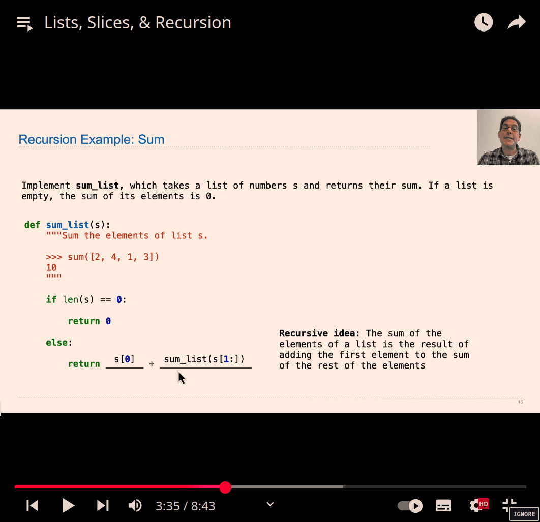
-
return s[0] + fn(s[1:])adding the first element to the sum of the rest of the element -
normal recursion using n-1 etc , this just adjust the slice number
tree recursion
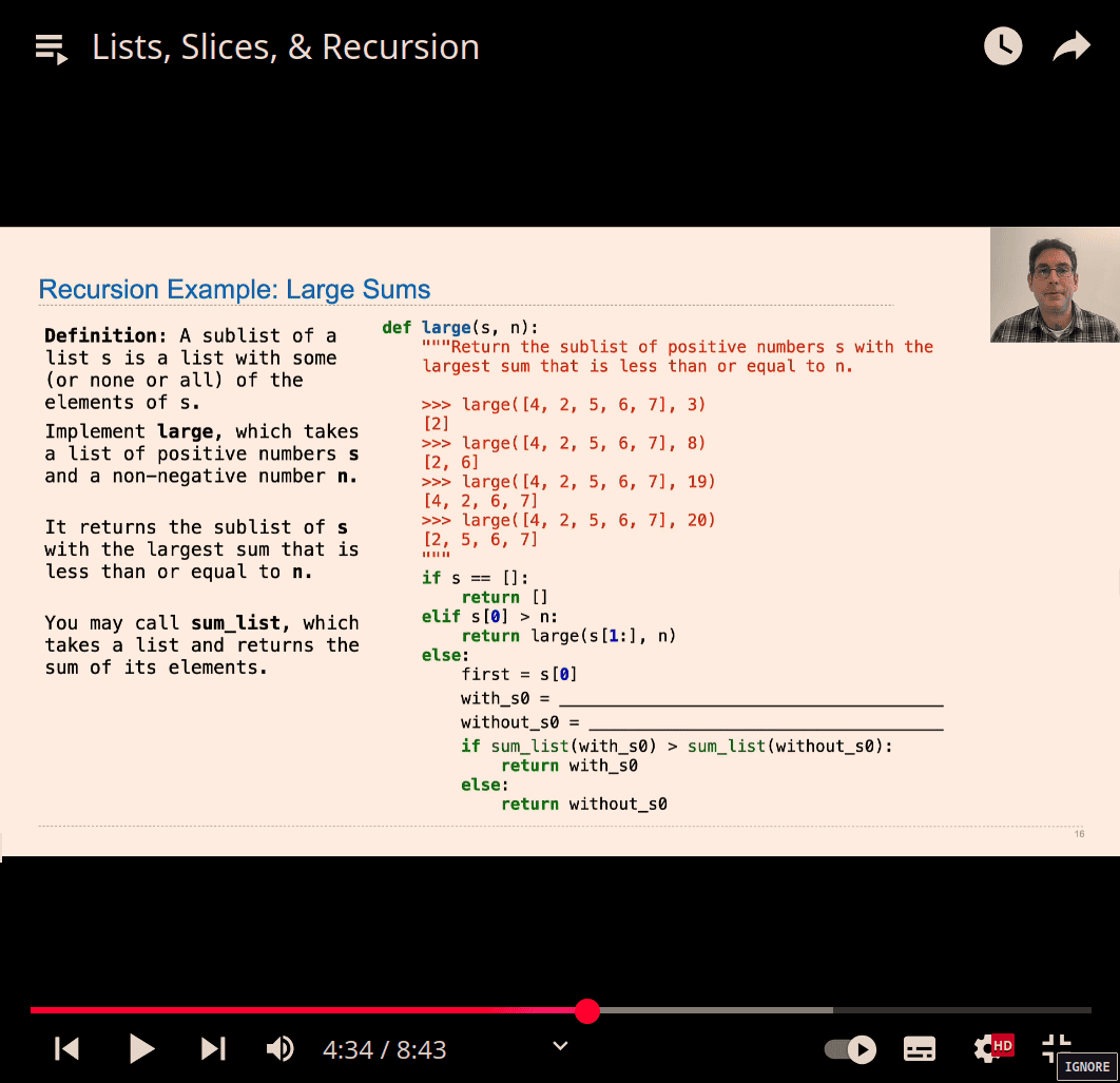
similar to previous problem?:
def count_partitions(n, m):
    if n == 0:
        return 1
    elif n < 0:
        return 0
    elif m == 0:
        return 0
    else:
        with_m = count_partitions(n - m, m)
        without_m = count_partitions(n, m - 1)
        return with_m + without_m
- nope
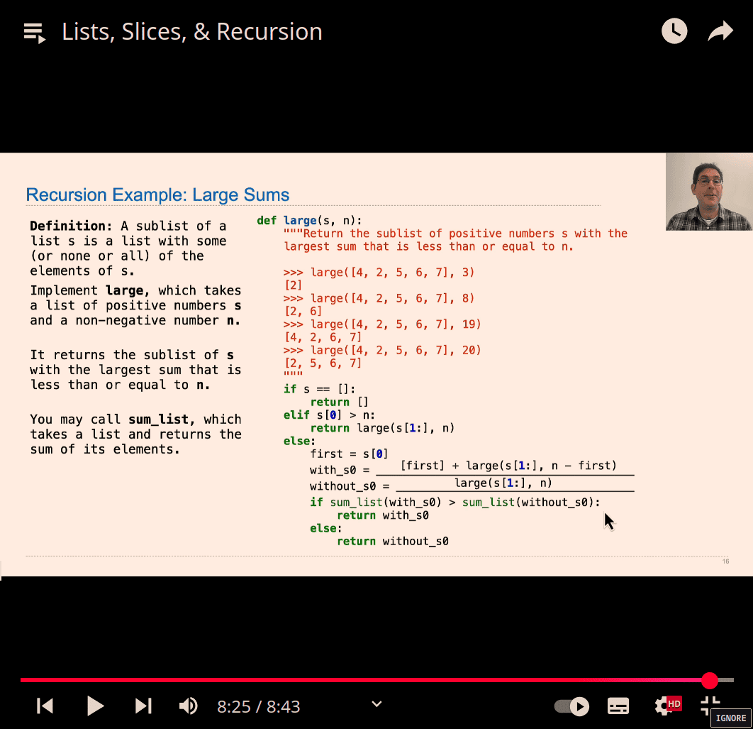
next chapter : (162) Box-and-Pointer Notation - YouTube
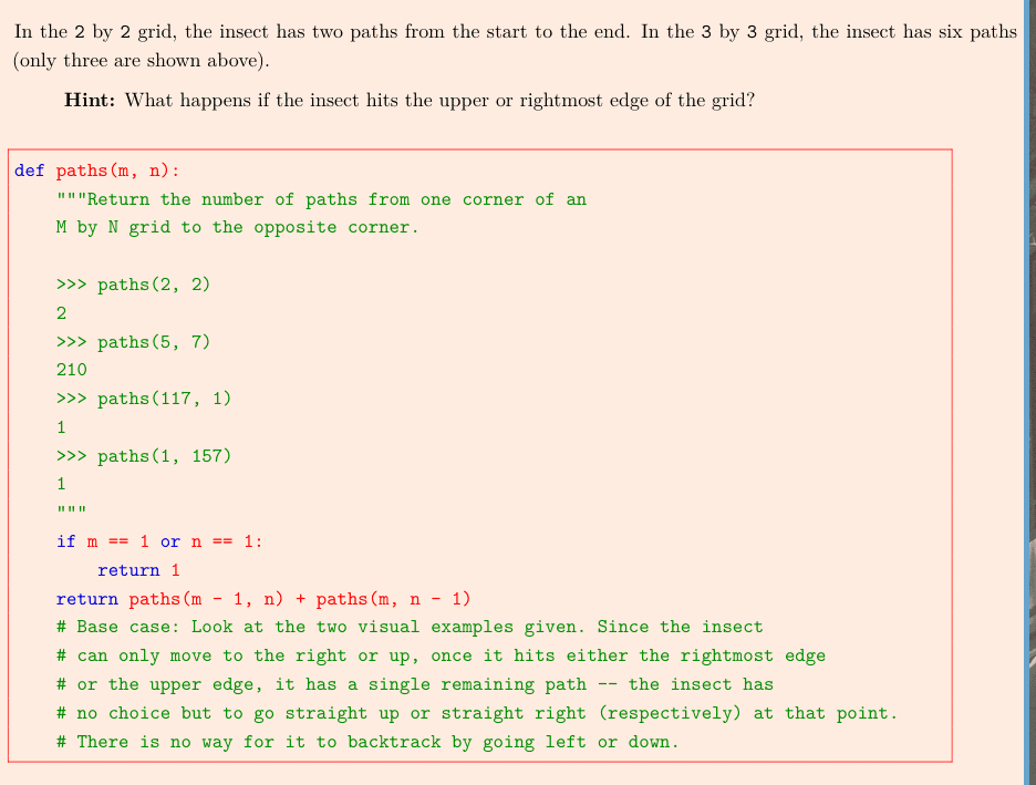
tree recusion dis:
 The most important thing to remember about lists is that a non-empty list s can be split into its first element s[0] and the rest of the list s[1:].
>>> s = [2, 3, 6, 4]
>>> s[0]
2
>>> s[1:]
[3, 6, 4]

using these to learn frist rather than append
sums(n,m)
n = total
m = max
return [all list]
q2
def max_product(s):
    """Return the maximum product of non-consecutive elements of s.

    >>> max_product([10, 3, 1, 9, 2])   # 10 * 9
    90
    >>> max_product([5, 10, 5, 10, 5])  # 5 * 5 * 5
    125
    >>> max_product([])                 # The product of no numbers is 1
    1
    """
Good question! Let’s break it down and understand why s[1:] * max_product(s[1+2:]) is incorrect, while non_first = max_product(s[1:]) is correct.
Understanding the “non-first” case
The goal of the “non-first” choice is to skip the first element and find the best product from the rest of the list.
Why is this wrong?
non_first = s[1:] * max_product(s[1+2:])-
Issue with Multiplication (
s[1:] * something)s[1:]is a list, not a single number.- You cannot multiply a list by a number like this; it’s a type error.
-
Incorrect Skipping Logic
s[1+2:]skips two elements froms[1:], but the “non-first” case only means skipping the first element.- You should not force skipping another element in this case.
Why is this correct?
non_first = max_product(s[1:])-
It correctly skips only the first element
- The purpose of “non-first” is just to ignore the first element and continue processing the rest normally.
- We pass
s[1:](everything except the first element) tomax_product(), letting the function decide the best product from there.
-
Recursive structure remains intact
max_product(s[1:])naturally handles choosing whether to include elements ats[1]or not.- No need to manually skip more elements.
Example Breakdown
Example: s = [10, 3, 1, 9, 2]
Let’s see how each approach behaves.
Your incorrect approach
non_first = s[1:] * max_product(s[1+2:]) # Incorrect!s[1:] = [3, 1, 9, 2]max_product(s[1+2:]) = max_product([9, 2])- But
s[1:] * max_product([9, 2])is invalid becauses[1:]is a list, and we cannot multiply a list by a number.
Correct approach
non_first = max_product(s[1:])- We correctly pass
[3, 1, 9, 2]intomax_product(), letting it handle the computation recursively.
Final Takeaway
- The “first” case involves multiplying because we actively pick an element.
- The “non-first” case just moves forward without multiplying, letting recursion handle it.
- Don’t manually skip extra elements for “non-first”; just call
max_product(s[1:]).
Does this explanation help? 😊
# Official (alternative) version
return max(s[0] * max_product(s[2:]), s[1] * max_product(s[3:]))
🔍 Key Difference:
Instead of just skipping the first element, the official version tries both:
- Taking
s[0]and skippings[1] - Taking
s[1]and skippings[2]
✅ Why it’s valid:
This version is exploring more options, not just one recursive path. It’s still selecting non-consecutive elements, but now it considers:
- What if we start by skipping the first element, and then pick
s[1]?
It might give a better product in some cases.
🧠 Summary:
- Your version is recursive and safe:
max(s[0]*..., max_product(s[1:])) - The alternative tries both
s[0]ands[1]as starting points.
Both are valid; the official one explores a broader search space.
Want to see an example where this difference matters?
- official ans→ no need using +1, just
[0:] and [2:] & [1] and [3]🔥
def sums(n, m):
    """Return lists that sum to n containing positive numbers up to m that
    have no adjacent repeats.

    >>> sums(5, 1)
    []
    >>> sums(5, 2)
    [[2, 1, 2]]
    >>> sums(5, 3)
    [[1, 3, 1], [2, 1, 2], [2, 3], [3, 2]]
    >>> sums(5, 5)
    [[1, 3, 1], [1, 4], [2, 1, 2], [2, 3], [3, 2], [4, 1], [5]]
    >>> sums(6, 3)
    [[1, 2, 1, 2], [1, 2, 3], [1, 3, 2], [2, 1, 2, 1], [2, 1, 3], [2, 3, 1], [3, 1, 2], [3, 2, 1]]
    """
    if n < 0:
        return []
    if n == 0:
        sums_to_zero = []     # The only way to sum to zero using positives
        return [sums_to_zero] # Return a list of all the ways to sum to zero
    result = []
    for k in range(1, m + 1):
        result = result + [ ___ for rest in ___ if rest == [] or ___ ]
    return result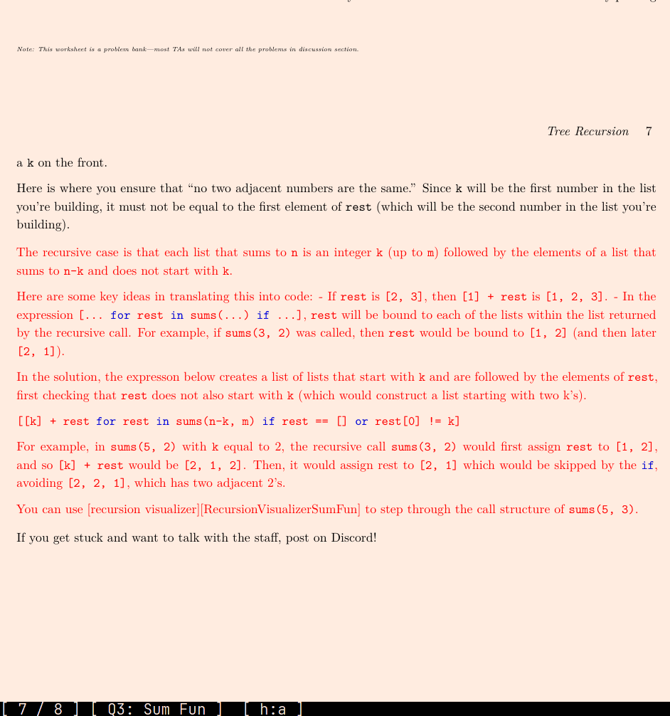
📌 Line in Question:
result = result + [[k] + rest for rest in sums(n - k, m) if rest == [] or rest[0] != k]🧠 First, let’s understand the goal
We’re trying to build all possible lists of numbers that:
- Add up to
n - Use only numbers
1tom - Have no adjacent duplicates
🧱 Break the line into smaller parts:
Part 1: The loop
for rest in sums(n - k, m)This is the recursive part.
- We already chose a number
k(in a loop from1tom) - So we subtract
kfrom the target:n - k - And we ask: What are all the valid lists that sum to
n - k? - Those results are stored in
rest
So rest is a valid list after we’ve already picked k
Part 2: The condition
if rest == [] or rest[0] != kThis is the adjacent repeat check.
- We don’t want to allow something like
[2, 2, 1] - So we check:
- If
restis empty ([]) → OK, there’s nothing to compare - Otherwise: make sure
rest[0] != k, sokisn’t repeated
- If
✅ Example:
Say k = 2 and rest = [2, 1], then:
rest[0] == k→ ❌ skip it (would give[2, 2, 1], which has adjacent2s)
Say rest = [1, 2]:
rest[0] != k→ ✅ keep it (result would be[2, 1, 2])
Part 3: The result building
[[k] + rest ...]Once we know rest is valid:
- We add
kto the front of it →[k] + rest - That’s one of our valid result lists
Part 4: Append to final list
result = result + ...We’re collecting all valid combinations, so we keep adding to result
✅ Final Visual Summary:
For every number k from 1 to m:
- Get all valid sublists that sum to
n - k - For each one:
- If it doesn’t start with
k, then:- Add
kin front - Save it in the final list
- Add
- If it doesn’t start with
🧪 Tiny Example:
sums(3, 2) — we want to find all valid lists of 1s and 2s that add up to 3, no adjacent repeats.
Here’s what would happen:
-
Try
k = 1n - k = 2- Call
sums(2, 2)→ maybe gives[[2], [1, 1]] - Check: can we put 1 in front?
[1, 1]❌ skip (1 == 1)[2]✅ keep →[1, 2]
-
Try
k = 2n - k = 1- Call
sums(1, 2)→ maybe gives[[1]] - Can we put 2 in front?
[1]✅ →[2, 1]
✅ Final result: [[1, 2], [2, 1]]
Let me know if you’d like this rewritten as a for-loop version — sometimes that’s easier to read than list comprehensions.
sums(5, 3):
    sums(4, 3):
        sums(3, 3):
            sums(2, 3):
                sums(1, 3):
                    sums(0, 3):
                    sums(0, 3) -> [[]]
                    sums(-1, 3):
                    sums(-1, 3) -> []
                    sums(-2, 3):
                    sums(-2, 3) -> []
                sums(1, 3) -> [[1]]
                sums(0, 3):
                sums(0, 3) -> [[]]
                sums(-1, 3):
                sums(-1, 3) -> []
            sums(2, 3) -> [[2]]
            sums(1, 3):
                sums(0, 3):
                sums(0, 3) -> [[]]
                sums(-1, 3):
                sums(-1, 3) -> []
                sums(-2, 3):
                sums(-2, 3) -> []
            sums(1, 3) -> [[1]]
            sums(0, 3):
            sums(0, 3) -> [[]]
        sums(3, 3) -> [[1, 2], [2, 1], [3]]
        sums(2, 3):
            sums(1, 3):
                sums(0, 3):
                sums(0, 3) -> [[]]
                sums(-1, 3):
                sums(-1, 3) -> []
                sums(-2, 3):
                sums(-2, 3) -> []
            sums(1, 3) -> [[1]]
            sums(0, 3):
            sums(0, 3) -> [[]]
            sums(-1, 3):
            sums(-1, 3) -> []
        sums(2, 3) -> [[2]]
        sums(1, 3):
            sums(0, 3):
            sums(0, 3) -> [[]]
            sums(-1, 3):
            sums(-1, 3) -> []
            sums(-2, 3):
            sums(-2, 3) -> []
        sums(1, 3) -> [[1]]
    sums(4, 3) -> [[1, 2, 1], [1, 3], [3, 1]]
    sums(3, 3):
        sums(2, 3):
            sums(1, 3):
                sums(0, 3):
                sums(0, 3) -> [[]]
                sums(-1, 3):
                sums(-1, 3) -> []
                sums(-2, 3):
                sums(-2, 3) -> []
            sums(1, 3) -> [[1]]
            sums(0, 3):
            sums(0, 3) -> [[]]
            sums(-1, 3):
            sums(-1, 3) -> []
        sums(2, 3) -> [[2]]
        sums(1, 3):
            sums(0, 3):
            sums(0, 3) -> [[]]
            sums(-1, 3):
            sums(-1, 3) -> []
            sums(-2, 3):
            sums(-2, 3) -> []
        sums(1, 3) -> [[1]]
        sums(0, 3):
        sums(0, 3) -> [[]]
    sums(3, 3) -> [[1, 2], [2, 1], [3]]
    sums(2, 3):
        sums(1, 3):
            sums(0, 3):
            sums(0, 3) -> [[]]
            sums(-1, 3):
            sums(-1, 3) -> []
            sums(-2, 3):
            sums(-2, 3) -> []
        sums(1, 3) -> [[1]]
        sums(0, 3):
        sums(0, 3) -> [[]]
        sums(-1, 3):
        sums(-1, 3) -> []
    sums(2, 3) -> [[2]]
sums(5, 3) -> [[1, 3, 1], [2, 1, 2], [2, 3], [3, 2]]
[[1, 3, 1], [2, 1, 2], [2, 3], [3, 2]]
Let’s take an easy example:
👉 sums(3, 2)
So:
- We want all combinations of 1s and 2s
- That sum to
3 - And don’t have adjacent repeats
🔁 Step-by-step with simple loops
Let’s write the logic more clearly using regular loops:
def sums(n, m):
    if n < 0:
        return []
    if n == 0:
        return [[]]  # Only one way to sum to zero

    result = []
    for k in range(1, m + 1):  # Try every number from 1 to m
        sublists = sums(n - k, m)  # Recursive call
        for rest in sublists:
            if rest == [] or rest[0] != k:  # No repeats
                result.append([k] + rest)   # Build the new list
    return result
🧠 What happens to rest?
Let’s trace sums(3, 2) step by step.
First call: sums(3, 2)
Try k = 1:
- Call
sums(2, 2)
Second call: sums(2, 2)
Try k = 1 again:
- Call
sums(1, 2)
Third call: sums(1, 2)
Try k = 1:
- Call
sums(0, 2)→ returns[[]] - Now we loop over
rest in [[]]rest = []→ ✅ pass the check- Add
[1] + []→[1]✅
Now sums(1, 2) → has [ [1] ] so far.
Try k = 2:
- Call
sums(-1, 2)→ returns[]
So done here.
Return: sums(1, 2) → [[1]]
Back to sums(2, 2)
Now we’re still handling k = 1, and sums(1, 2) returned [[1]]
We loop:
rest = [1]- Check: is
rest[0] != k? →1 == 1❌ skip it!
Now try k = 2:
- Call
sums(0, 2)→ returns[[]]
Loop:
rest = []→ ✅- Add
[2] + []→[2]
Return: sums(2, 2) → [[2]]
Back to sums(3, 2)
We’re at k = 1, and sums(2, 2) gave [[2]]
Loop:
rest = [2]→2 != 1✅- Add
[1] + [2]→[1, 2]
Now try k = 2:
- Call
sums(1, 2)→ returned[[1]]
Loop:
rest = [1]→1 != 2✅- Add
[2] + [1]→[2, 1]
✅ Final result of sums(3, 2):
[[1, 2], [2, 1]]
🔄 How rest changes
It’s the result of the recursive call each time:
sums(0, 2)→[[]]sums(1, 2)→[[1]]sums(2, 2)→[[2]]sums(3, 2)builds on that to form[1, 2],[2, 1]
Each time you add a number k, you get smaller problems, and rest is the partial solution to that smaller problem.
TL;DR:
restis a partial solution from a recursive call- You’re trying to build on
restby adding a new numberkin front - But you skip it if
rest[0] == kto avoid adjacent repeats
Awesome — let’s visualize the recursive calls of sums(3, 2) as a tree diagram 🌲, so you can clearly see how the recursion works, how rest is built, and how adjacent repeats are avoided.
📌 Problem: sums(3, 2)
We want to find all the non-repeating adjacent sequences of numbers 1 to 2 that sum to 3.
🌲 Tree of Recursive Calls
We’ll show it like:
current_call (n)
├── try k = 1
│   └── recursive call: sums(n - 1, m)
└── try k = 2
    └── recursive call: sums(n - 2, m)
Root: sums(3, 2)
sums(3, 2)
├── k = 1 → sums(2, 2)
│   ├── k = 1 → sums(1, 2)
│   │   ├── k = 1 → sums(0, 2) ✅ returns [[]]
│   │   └── k = 2 → sums(-1, 2) ❌ invalid
│   │   → builds: [1] + [] = [1] ✅
│   │   → return: [[1]]
│   └── k = 2 → sums(0, 2) ✅ returns [[]]
│       → builds: [2] + [] = [2] ✅
│   → Now from `sums(2, 2)` we have: [[2]], because [1] is invalid (adj repeat with prev 1)
│   → Back to `sums(3, 2)`, build: [1] + [2] = [1, 2] ✅
├── k = 2 → sums(1, 2)
│   ├── k = 1 → sums(0, 2) ✅ returns [[]]
│   │   → builds: [1] + [] = [1] ✅
│   └── k = 2 → sums(-1, 2) ❌ invalid
│   → Return: [[1]]
│   → Back to `sums(3, 2)`, build: [2] + [1] = [2, 1] ✅
✅ Final Result:
From root sums(3, 2), we got:
[1, 2][2, 1]
So:
sums(3, 2) → [[1, 2], [2, 1]]🔁 And how rest changes:
| Call | Returned rest | Built [k] + rest | Keep or Skip |
|---|---|---|---|
sums(0, 2) | [[]] | [1], [2] | ✅ |
sums(1, 2) | [[1]] | [1, 1], [2, 1] | ❌, ✅ |
sums(2, 2) | [[2]] | [1, 2] | ✅ |
Let me know if you want to go one level deeper (e.g., sums(4, 2) tree) or see it as a visual chart!
Project2
Let’s analyze the provided implementation of the choose function (which seems to be equivalent to the pick function from your earlier question) and compare it to the approach we discussed. Then, I’ll explain why the author initializes count = -1 and explore an alternative approach, highlighting the differences.
Provided Implementation:
def choose(paragraphs, select, k):
    """Return the Kth paragraph from PARAGRAPHS for which SELECT called on the
    paragraph returns true. If there are fewer than K such paragraphs, return
    the empty string.
    """
    count = -1
    for p in paragraphs:
        if select(p):
            count += 1
            if count == k:
                return p
    return ""
How It Works:
- Initialization:
count = -1- Starts the counter at
-1instead of0.
- Starts the counter at
- Loop: Iterates over
paragraphsdirectly (usingpinstead of indices). - Condition: When
select(p)isTrue:- Increments
count(from-1to0on the first valid paragraph, then1, etc.). - Checks if
count == k. If true, returns the current paragraphp.
- Increments
- Default Return: If the loop ends (i.e., not enough valid paragraphs), returns
''.
Testing with Example:
ps = ['short', 'really long', 'tiny']s = lambda p: len(p) <= 5k = 2'short':len = 5,True,count = -1 + 1 = 0(not 2, continue)'really long':len = 11,False,countstays0'tiny':len = 4,True,count = 0 + 1 = 1(not 2, continue)- End:
count = 1, fewer thank = 2valid paragraphs, returns''.
This matches the expected behavior.
Alternative Approach (from Earlier):
Here’s the version we discussed previously:
def pick(paragraphs, select, k):
    count = 0
    for i in range(len(paragraphs)):
        if select(paragraphs[i]):
            if count == k:
                return paragraphs[i]
            count += 1
    return ''
Differences:
-
Starting Value of
count:- Provided (
count = -1): Starts at-1and increments before checking againstk. - Alternative (
count = 0): Starts at0and increments after checking againstk.
- Provided (
-
Order of Operations:
- Provided: Increments
countfirst, then checks if it equalsk. This meanscountrepresents the index of the current valid paragraph after incrementing. - Alternative: Checks
count == kfirst, then increments. Here,countrepresents how many valid paragraphs have been seen before the current one.
- Provided: Increments
-
Loop Style:
- Provided: Uses
for p in paragraphs(direct iteration over elements). - Alternative: Uses
for i in range(len(paragraphs))(iteration over indices).
- Provided: Uses
Why count = -1?
The choice of count = -1 is a subtle but intentional design decision:
- Logic: By starting at
-1, the first valid paragraph incrementscountto0, the second to1, and so on. Whencount == k, it’s naturally aligned with the 0-based index of thekth valid paragraph (e.g.,k = 0is the 0th valid paragraph,k = 1is the 1st, etc.). - Simplicity: This allows the increment and comparison to happen in one clean step inside the
if select(p)block, avoiding an extra condition or adjustment elsewhere. - Example:
k = 0(first valid paragraph):'short':count = -1 + 1 = 0,0 == 0, returns'short'.
k = 1:'short':count = -1 + 1 = 0,0 != 1, continue'tiny':count = 0 + 1 = 1,1 == 1, returns'tiny'.
If it started at 0 and incremented first, you’d need to adjust the comparison (e.g., count - 1 == k), which adds complexity.
Another Way to Do It:
Here’s an alternative that avoids the -1 trick by using a different structure:
def choose(paragraphs, select, k):
    valid_paragraphs = [p for p in paragraphs if select(p)]  # Filter valid paragraphs
    return valid_paragraphs[k] if k < len(valid_paragraphs) else ''
How It Works:
- List Comprehension: Creates a list of all paragraphs where
select(p)isTrue. - Indexing: Returns the
kth element if it exists, otherwise''.
Differences:
- Efficiency: Less efficient for large lists because it processes the entire list upfront, even if
kis small (e.g.,k = 0). The other versions stop as soon as they find thekth match. - Readability: More concise and arguably easier to understand at a glance.
- Memory: Uses more memory by storing the filtered list, whereas the loop versions don’t.
Example:
ps = ['short', 'really long', 'tiny']s = lambda p: len(p) <= 5k = 2valid_paragraphs = ['short', 'tiny']len(valid_paragraphs) = 2,k = 2 >= 2, returns''.
Why count = -1 vs. count = 0?
count = -1: Aligns the increment with the index naturally, making the logic flow smoothly without extra adjustments. It’s a common pattern when you want the counter to match the current item’s position after processing.count = 0: Requires incrementing after the check, which works but separates the “found it” logic from the counter update. It’s more intuitive if you think ofcountas “how many I’ve seen so far.”
Both are correct, but count = -1 is slightly more elegant here because it avoids an extra line or condition. The list comprehension alternative trades elegance for simplicity but sacrifices early termination.
Does this clarify the differences and reasoning? Let me know if you’d like to explore further!
def about(topic):
    """Return a select function that returns whether a paragraph contains one
    of the words in TOPIC.

    >>> about_dogs = about(['dog', 'dogs', 'pup', 'puppy'])
    >>> choose(['Cute Dog!', 'That is a cat.', 'Nice pup!'], about_dogs, 0)
    'Cute Dog!'
    >>> choose(['Cute Dog!', 'That is a cat.', 'Nice pup.'], about_dogs, 1)
    'Nice pup.'
    """
    assert all([lower(x) == x for x in topic]), 'topics should be lowercase.'
    # BEGIN PROBLEM 2
    "*** YOUR CODE HERE ***"
    def select(paragraph):
        words = set(split(lower(remove_punctuation(paragraph))))
        for x in topic:
            if x in words:
                return True
        return False
    return select
    # END PROBLEM 2
   # other method :
    def about2(text):
            text1 = remove_punctuation(text)
            text2 = split(text1)
            text2_low = [lower(x) for x in text2]

            subject_low = [lower(x) for x in subject]

            for i in subject_low:
                for j in text2_low:
                    if i == j:
                        return True
            return False
    return about2
"""Return the accuracy (percentage of words typed correctly) of TYPED
when compared to the prefix of REFERENCE that was typed.

>>> accuracy('Cute Dog!', 'Cute Dog.')
50.0
>>> accuracy('A Cute Dog!', 'Cute Dog.')
0.0
>>> accuracy('cute Dog.', 'Cute Dog.')
50.0
>>> accuracy('Cute Dog. I say!', 'Cute Dog.')
50.0
>>> accuracy('Cute', 'Cute Dog.')
100.0
>>> accuracy('', 'Cute Dog.')
0.0
unit reference/typed
length
saniterize
"""
    a = len(typed_words)
    b = len(source_words)
    if  a == 0 and b == 0 :
        return 100.0
    elif a == 0 or b == 0 :
        return 0.0

    count = 0
    for i in range(0, a):
        if i+1 > b:
            break
        elif typed_words[i] == source_words[i]:
            count += 1
    return count * 100 / a

def accuracy(typed, reference):
    typed_words = split(typed)
    reference_words = split(reference)
    # BEGIN PROBLEM 3
    "*** YOUR CODE HERE ***"
    if len(typed_words) == 0 and len(source_words) == 0:
        return 100.0
    elif len(typed_words) == 0:
        return 0.0

    correct = 0
    for x, y in zip(typed_words, source_words):
        if x == y:
            correct += 1

    return correct / len(typed_words) * 100.0

    # END PROBLEM 3
- return correct / len(typed_words) * 100.0
Let’s dive into comparing these two implementations of the accuracy function, analyze their differences, determine which one is “better” based on the problem requirements, and explain how zip works in the first solution. We’ll evaluate correctness, readability, and efficiency, and then tie it all back to the problem’s intent.
Problem Recap:
- Function:
accuracy(typed, source) - Purpose: Calculate the percentage of words in
typedthat correctly match the corresponding words in the prefix ofsource. - Inputs:
typed: A string that may contain typos.source: A reference string without errors.
- Output: A float (0.0 to 100.0) representing the percentage of correctly typed words.
- Assumptions:
splitis a helper function (not shown) that splits a string into a list of words (e.g.,'Cute Dog!'→['Cute', 'Dog!']).
Test Cases:
accuracy('Cute Dog!', 'Cute Dog.')→50.0(1/2 words correct)accuracy('A Cute Dog!', 'Cute Dog.')→0.0(no matches in prefix)accuracy('cute Dog.', 'Cute Dog.')→50.0(1/2 correct, case-sensitive)accuracy('Cute Dog. I say!', 'Cute Dog.')→50.0(1/2 correct in prefix)accuracy('Cute', 'Cute Dog.')→100.0(1/1 correct)accuracy('', 'Cute Dog.')→0.0accuracy('', '')→100.0
Solution 1: Using zip
def accuracy(typed, source):
    typed_words = split(typed)
    reference_words = split(source)  # Note: 'reference_words' should be 'source_words'
    if len(typed_words) == 0 and len(reference_words) == 0:
        return 100.0
    elif len(typed_words) == 0:
        return 0.0

    correct = 0
    for x, y in zip(typed_words, reference_words):
        if x == y:
            correct += 1

    return correct / len(typed_words) * 100.0
How It Works:
- Base Cases:
- If both
typedandsourceare empty →100.0. - If
typedis empty butsourceisn’t →0.0.
- If both
- Main Logic:
- Uses
zipto pair words fromtyped_wordsandreference_words(should besource_words—a naming inconsistency). - Counts matches with
correct. - Returns
(correct / len(typed_words)) * 100.
- Uses
How zip Works:
zip(typed_words, source_words)creates an iterator of tuples, pairing elements from both lists up to the length of the shorter list.- Example:
typed_words = ['Cute', 'Dog!']source_words = ['Cute', 'Dog.']zip→[('Cute', 'Cute'), ('Dog!', 'Dog.')]- If
typed_words = ['A', 'Cute', 'Dog!']andsource_words = ['Cute', 'Dog.'],zip→[('A', 'Cute'), ('Cute', 'Dog.')].
for x, y in zip(...)unpacks each pair, comparingx(fromtyped) andy(fromsource).
Pros:
- Concise:
ziphandles pairing automatically. - Readable: The intent (comparing corresponding words) is clear.
Cons:
- Naming Bug: Uses
reference_wordsinternally butsource_wordsshould be consistent with the parametersource. - Incomplete Base Case: Doesn’t check
len(source_words) == 0whentyped_wordsisn’t empty, which could lead to division by zero or incorrect behavior ifsourceis empty buttypedisn’t.
Solution 2: Using Index-Based Loop
def accuracy(typed, source):
    typed_words = split(typed)
    source_words = split(source)
    a = len(typed_words)
    b = len(source_words)
    if a == 0 and b == 0:
        return 100.0
    elif a == 0 or b == 0:
        return 0.0

    count = 0
    for i in range(0, a):
        if i + 1 > b:
            break
        elif typed_words[i] == source_words[i]:
            count += 1
    return count * 100 / a
How It Works:
- Base Cases:
- Both empty →
100.0. - Either empty →
0.0(coverstypedempty orsourceempty).
- Both empty →
- Main Logic:
- Loops over indices of
typed_words(up toa). - Checks if index
iexceedssource_wordslength (b) to avoid index errors. - Compares words at matching indices, increments
countfor matches. - Returns
(count / a) * 100.
- Loops over indices of
Pros:
- Robust Base Case: Handles all empty scenarios explicitly.
- Prefix Focus: Stops comparing when
source_wordsruns out, aligning with “prefix ofsource” requirement.
Cons:
- Verbose: Manual index checking is less elegant than
zip. - Potential Confusion:
i + 1 > bcould be written asi >= bfor clarity (sinceiis 0-based).
Key Differences:
-
Handling
sourceShorter thantyped:- Zip: Automatically stops at the shorter list. If
source_wordsis shorter, it ignores extratyped_words, which aligns with “prefix ofsource”. - Index: Explicitly breaks when
i >= b, achieving the same result.
- Zip: Automatically stops at the shorter list. If
-
Base Case Completeness:
- Zip: Misses
len(source_words) == 0whentyped_wordsisn’t empty (e.g.,'Cute'vs.''). This should return0.0, but it attempts division by zero or incorrect logic. - Index: Covers all cases with
a == 0 or b == 0.
- Zip: Misses
-
Style:
- Zip: More Pythonic, leveraging built-in tools.
- Index: More manual, but explicit.
Which is Better?
- Correctness: Solution 2 (Index) is more robust due to its complete base case handling. Solution 1 (Zip) has a bug when
sourceis empty buttypedisn’t, potentially causing runtime errors or incorrect results unless fixed. - Readability: Solution 1 (Zip) wins for conciseness and elegance, assuming the base case is corrected.
- Efficiency: Both are O(min(n, m)) where
n = len(typed_words),m = len(source_words), so no significant difference.
Fixed Zip Version:
def accuracy(typed, source):
    typed_words = split(typed)
    source_words = split(source)
    if len(typed_words) == 0 and len(source_words) == 0:
        return 100.0
    if len(typed_words) == 0 or len(source_words) == 0:
        return 0.0
    correct = 0
    for x, y in zip(typed_words, source_words):
        if x == y:
            correct += 1
return correct / len(typed_words) * 100.0- Adds
len(source_words) == 0check. - Now fully correct and more readable than the index version.
Conclusion:
- Best Choice: The fixed
zipversion is better because it’s:- Correct: Handles all edge cases.
- Readable: Uses Python’s
zipfor a clean, idiomatic solution. - Maintainable: Less prone to manual errors like index mismanagement.
- Why
zipWorks Well Here: It naturally aligns with comparing two sequences positionally up to the shorter length, perfectly matching the “prefix ofsource” requirement.
Let me know if you’d like to explore further or test more edge cases!
def wpm(typed, elapsed):
    """Return the words-per-minute (WPM) of the TYPED string.

    Arguments:
        typed: an entered string
        elapsed: an amount of time in seconds

    >>> wpm('hello friend hello buddy hello', 15)
    24.0
    >>> wpm('0123456789',60)
    2.0
    """
    assert elapsed > 0, "Elapsed time must be positive"
    # BEGIN PROBLEM 4
    "*** YOUR CODE HERE ***"
    length = len(typed)
    rate = 60 / elapsed
    return length * rate / 5
    # END PROBLEM 4
Let’s dive into these two implementations of the autocorrect function, break down their concepts, and compare how they solve the same problem in different ways. I’ll explain the logic behind each approach, highlight their strengths and weaknesses, and clarify why they both work (or don’t) for the given test cases. This will help you understand the problem-solving strategies and trade-offs involved.
Problem Recap
- Goal: Return the word from
word_list(orvalid_words) with the smallest difference fromtyped_word, as measured bydiff_function. If the smallest difference exceedslimit, returntyped_word. If multiple words tie for the smallest difference, return the first one in the list. - Inputs:
typed_word: A string (e.g.,"hwllo").word_list/valid_words: A list of strings (e.g.,["butter", "hello", "potato"]).diff_function: A function returning a number representing the difference between two words.limit: A number (e.g.,20).
- Test Cases:
autocorrect("hwllo", ["butter", "hello", "potato"], ten_diff, 20)→'butter'autocorrect("tosting", ["testing", "asking", "fasting"], first_diff, 10)→'testing'
Solution 1: Iterative with Early Initialization
def autocorrect(typed_word, word_list, diff_function, limit):
    min_diff = limit + 1
    best_word = typed_word

    for word in word_list:
        if word == typed_word:
            return typed_word

        diff = diff_function(typed_word, word, limit)

        if min_diff > abs(diff):
            min_diff = abs(diff)
            best_word = word

    return typed_word if min_diff > limit else best_word
Concept Explained:
- Initialization:
min_diff = limit + 1: Starts higher thanlimitso that if no word is better,typed_wordis returned by default.best_word = typed_word: Pre-sets the fallback return value, avoiding extra logic later.
- Early Exit:
if word == typed_word: If the exact word is inword_list, return it immediately. This optimizes for the case where no correction is needed.
- Loop Logic:
- Computes
difffor each word usingdiff_function. - Uses
abs(diff)to handle potential negative differences (though test cases suggest non-negative outputs). - Updates
min_diffandbest_wordif the newdiffis smaller (using>ensures the first tied word is kept).
- Computes
- Final Decision:
- Ternary expression: Returns
typed_wordifmin_diff > limit, otherwisebest_word.
- Ternary expression: Returns
How It Works with Test Cases:
"hwllo",["butter", "hello", "potato"],ten_diff,20:min_diff = 21,best_word = "hwllo"."hwllo" not in list, no early return.diff(butter) = 10,21 > 10,min_diff = 10,best_word = "butter".diff(hello) = 10,10 > 10is false (tie), no update.diff(potato) = 10, no update.10 ≤ 20, return"butter".
"tosting",["testing", "asking", "fasting"],first_diff,10:min_diff = 11,best_word = "tosting"."tosting" not in list".diff(testing) = 0,11 > 0,min_diff = 0,best_word = "testing".diff(asking) = 1,0 > 1is false.diff(fasting) = 1, no update.0 ≤ 10, return"testing".
Key Concept:
- Single Pass with Default: It iterates once, updating the best candidate only when a strictly smaller difference is found, and defaults to
typed_wordif the limit is exceeded. Theabs(diff)adds flexibility for diff functions that might return negatives.
Solution 2: List Comprehension with Index Lookup
def autocorrect(typed_word, valid_words, diff_function, limit):
    if typed_word in valid_words:
        return typed_word
    diff_list = [diff_function(typed_word, word, limit) for word in valid_words]
    if min(diff_list) > limit:
        return typed_word
    else:
        return valid_words[diff_list.index(min(diff_list))]
Concept Explained:
- Early Exit:
if typed_word in valid_words: Similar to Solution 1, returnstyped_wordif it’s already valid.
- Compute All Differences:
diff_list = [diff_function(...)]: Uses a list comprehension to create a list of differences for all words invalid_words.
- Find Minimum and Decide:
min(diff_list): Finds the smallest difference.- If
min > limit, returnstyped_word. - Otherwise, uses
diff_list.index(min(diff_list))to find the first word with that minimum difference and returns it fromvalid_words.
How It Works with Test Cases:
"hwllo",["butter", "hello", "potato"],ten_diff,20:"hwllo" not in list".diff_list = [10, 10, 10].min(diff_list) = 10,10 ≤ 20.diff_list.index(10) = 0(first occurrence), return"butter".
"tosting",["testing", "asking", "fasting"],first_diff,10:"tosting" not in list".diff_list = [0, 1, 1].min(diff_list) = 0,0 ≤ 10.diff_list.index(0) = 0, return"testing".
Key Concept:
- Batch Processing: Computes all differences upfront, then processes them with built-in functions (
minandindex). It relies on Python’s list operations to handle ties (first occurrence by default).
Comparison of Concepts
1. Approach to Finding the Minimum
- Solution 1 (Iterative):
- Tracks the minimum difference incrementally in a single loop.
- Updates
best_wordonly when a strictly smaller difference is found (>). - Pros: Memory-efficient (no extra list), stops updating once the minimum stabilizes.
- Cons: Slightly more manual logic.
- Solution 2 (List Comprehension):
- Computes all differences into a list, then finds the minimum and its index.
- Pros: Cleaner, leverages Python’s built-ins.
- Cons: Uses more memory (stores
diff_list), less efficient for large lists.
2. Handling Ties
- Both satisfy “return the one closest to the front”:
- Solution 1: Uses
<(not<=), so ties don’t overwritebest_word, keeping the first. - Solution 2:
index(min())returns the first occurrence of the minimum naturally.
- Solution 1: Uses
3. Limit Check
- Solution 1: Integrates it into the return logic with a pre-set default (
typed_word). - Solution 2: Explicitly checks
min(diff_list) > limit, more declarative.
4. Early Exit
- Both check if
typed_wordis in the list, optimizing for exact matches.
5. Use of abs
- Solution 1: Applies
abs(diff)to handle potential negative differences. - Solution 2: Assumes non-negative differences (test cases support this).
- Note: Test cases (
ten_diff,first_diff) return non-negative values, soabsisn’t strictly necessary but adds robustness.
Which is Better?
- Correctness:
- Both work for the test cases.
- Solution 1’s
abs(diff)is overkill here but safer for untesteddiff_functions.
- Efficiency:
- Solution 1: O(n) time, O(1) space (n = len(word_list)).
- Solution 2: O(n) time for list creation, O(n) space for
diff_list, plus O(n) forindex, totaling O(n) time but higher memory. - Winner: Solution 1 for large lists.
- Readability:
- Solution 1: More explicit, but requires understanding the initialization trick (
limit + 1). - Solution 2: More concise and Pythonic, easier to read at a glance.
- Winner: Solution 2 for clarity.
- Solution 1: More explicit, but requires understanding the initialization trick (
- Maintainability:
- Solution 2’s list comprehension is easier to modify (e.g., for debugging or adding conditions).
Verdict:
- Solution 2 is better for small lists and readability, aligning with Python’s style.
- Solution 1 is preferable for performance with large lists or memory constraints.
Conceptual Takeaway
- Iterative (Solution 1): “Build the answer as you go.” Good for control and efficiency.
- Declarative (Solution 2): “Compute everything, then decide.” Good for simplicity and leveraging Python’s tools.
Both embody the core idea: minimize difference, respect the limit, and prioritize the first tie. Your choice depends on context (e.g., list size, coding style preference). Does this clarify the concepts? Let me know if you want to explore further!
extra info about diff
>>> def length_diff(w1, w2, limit):
...     return min(limit + 1, abs(len(w2) - len(w1)))
>>> length_diff('mellow', 'cello', 10)
1
>>> length_diff('hippo', 'hippopotamus', 5)
6